Example: Bang-bang Control
Double Integrator Minimum-Time Repositioning
Difficulty: Easy
The problem was adapted from Example 4.11 from [1].
Consider the system illustrated below
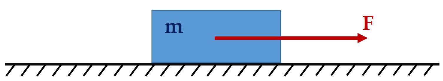
If we neglect viscous friction, consider a unit mass and let u=F, then the optimal control problem to find control input such that the object is repositioned from x=0 [m] to x=300 [m] in mimimum time will be

Subject to dynamics constraints

simple bounds on variables

and boundary conditions

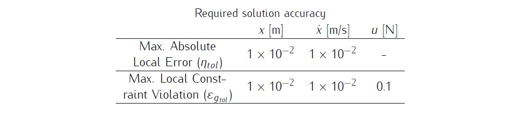
We require the numerical solution to fulfill the following accuracy criteria
Formulate the problem in ICLOCS2
In internal model defination file BangBang_Dynamics_Internal.m
We can specify the system dynamics in function BangBang_Dynamics_Internal with
x2 = x(:,2);
u1 = u(:,1);
dx(:,1) = x2;
dx(:,2) = u1;
For this example problem, we do not have any path constraints, so function BangBang_Dynamics_Internal only need to return the value of variable dx .
Similarly, the (optional) simulation dynamics can be specifed in function BangBang_Dynamics_Sim .
In problem defination file BangBang.m
First we provide the function handles for system dynamics with,
InternalDynamics=@BangBang_Dynamics_Internal;
SimDynamics=@BangBang_Dynamics_Sim;
the optional files providing analytic derivatives,
problem.analyticDeriv.gradCost=@gradCost_BangBang;
problem.analyticDeriv.hessianLagrangian=@hessianLagrangian_BangBang;
problem.analyticDeriv.jacConst=@jacConst_BangBang;
and the function handle for the settings file.
problem.settings=@settings_Bangbang;Next we define the time variables with
problem.time.t0_min=0;
problem.time.t0_max=0;
guess.t0=0;
and
problem.time.tf_min=0;
problem.time.tf_max=35;
guess.tf=30;
For state variables, we need to provide the initial conditions
problem.states.x0=[0 0];bounds on intial conditions
problem.states.x0l=[0 0];
problem.states.x0u=[0 0];
state bounds
problem.states.xl=[-10 -200];
problem.states.xu=[300 200];
bounds on the absolute local and global (integrated) discretization error of state variables
problem.states.xErrorTol_local=[1e-2 1e-2];
problem.states.xErrorTol_integral=[1e-2 1e-2];
tolerance for state variable box constraint violation
problem.states.xConstraintTol=[1e-2 1e-2];terminal state bounds
problem.states.xfl=[300 0];
problem.states.xfu=[300 0];
and an initial guess of the state trajectory (optional but recommended)
guess.states(:,1)=[0 300];
guess.states(:,2)=[0 0];
Lastly for control variables, we need to define simple bounds
problem.inputs.ul=[-2];
problem.inputs.uu=[1];
bounds on the first control action
problem.inputs.u0l=[-2];
problem.inputs.u0u=[1];
tolerance for control variable box constraint violation
problem.inputs.uConstraintTol=[0.1]; as well as an initial guess of the input trajectory (optional but recommended)
guess.inputs(:,1)=[1 -2];Since this problem only has a Mayer (boundary) cost , and no Lagrange (stage) cost ,we simply have
boundaryCost=tf;stageCost = 0*t;for sub-function E_unscaled and L_unscaled respectively.
For this example problem, we do not have additional boundary constraints (in addition to varialbe simple bounds). Thus we can leave routines b_unscaled as they are.
Analytical derivatives
The analytical derivatives for the problem can be supplied with the following additional files: gradCost_BangBang.m for cost gradient, jacConst_BangBang.m for constraint Jacobian, and hessianLagrangian_BangBang.m for the Lagrangian Hessian. Instructions on how to formulate these files are included in the function descriptions.
Main script main_Bangbang.m
Now we can fetch the problem and options, solve the resultant NLP, and generate some plots for the solution.
[problem,guess]=BangBang;          % Fetch the problem definition
options= problem.settings(30);                  % Get options and solver settings
[solution,MRHistory]=solveMyProblem( problem,guess,options);
genSolutionPlots(options, solution);
Results from ICLOCS2
Standard solve with mesh refinement
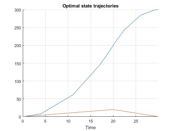
Using the 'AutoDirect' (Automatic chosen direct collocation) method of ICLOCS2, the following state and input trajectories are obtained after one mesh refinement iterations with the Hermite-Simpson discretization scheme. The graphs are generated by ICLOCS 2.5 built-in genSolutionPlots command.
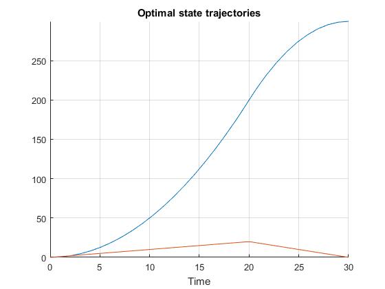
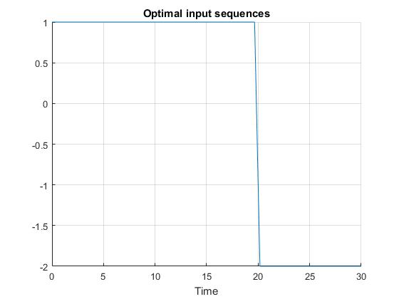
Starting from 30 equally spaced mesh points, it can be observed that additional mesh points are placed in the mesh refinement process to capture the control switching structure ('bang-bang' behavior). The computation time is about 0.7 seconds using analytical derivative calculations on an Intel i7-6700 desktop computer. Subsequent recomputation using the refined mesh and warm starting will take on average 0.2 seconds and 18 iterations.
Solve with flexible hp-adaptive mesh
For this problem, we may also use ICLOCS2's unique flexible hp-adaptive mesh to yield solution that better captures the switch of the input, without the need to add additional mesh points.
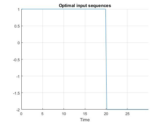
We start with four equally-spaced mesh points, each with a polynomial degree of four. As the NLP converges, the mesh intervals and collocation points start to gather around the control switching time instance, accurately capturing this discontinuity in the optimal solution at 20s.
[1] J. Betts, Practical Methods for Optimal Control and Estimation Using Nonlinear Programming: Second Edition, Advances in Design and Control, Society for Industrial and Applied Mathematics, 2010.