Example:
Aircraft Go-Around in the Presence of Windshear
Difficulty: Hard
The problem was initially presented by [1-2]. This implementation contain modifications to the original formulation by [3].
Consider following problem where a commerical aircraft encountered windshear during landing and need to go-around
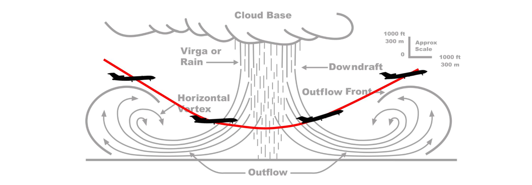
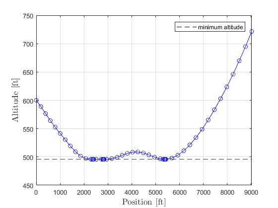
the objective is to maximize the lowest altitude ever reached

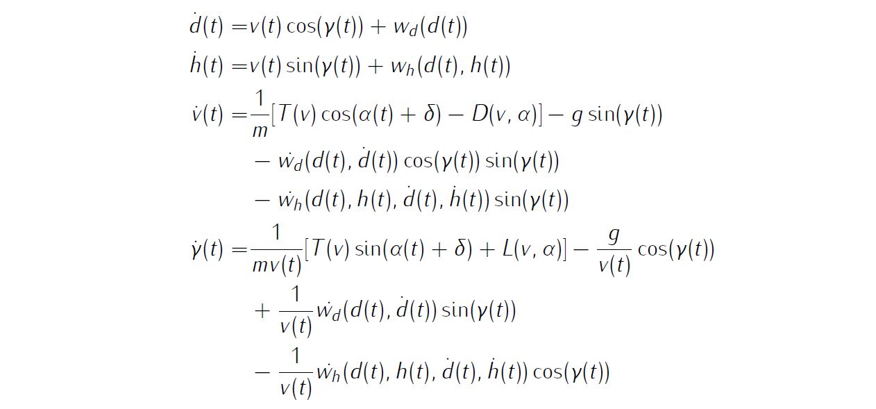
Subject to dynamics constraints
path constraint

simple bounds on variables

and boundary conditions

Details about the windshear, aerodynamic modelling as well as parameter values of all relevant variables are available in various references, thus will not be reproduced here.
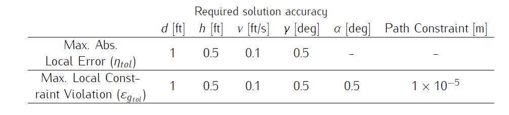
We require the numerical solution to fulfill the following accuracy criteria
Formulate the problem in ICLOCS2
In internal model defination file WindshearGoAround_Dynamics_Internal.m
We can specify the system dynamics in function WindshearGoAround_Dynamics_Internal with
auxdata = vdat.auxdata;

pos = x(:,1);
h = x(:,2);
v = x(:,3);
fpa = x(:,4);
alpha = u(:,1);

T=ppval(auxdata.beta_poly,t).*(auxdata.A_0+auxdata.A_1.*v+auxdata.A_2.*v.^2);
D=0.5*(auxdata.B_0+auxdata.B_1.*alpha+auxdata.B_2.*alpha.^2).*auxdata.rho.*auxdata.S.*v.^2;
L=0.5*ppval(auxdata.C_L_poly,alpha).*auxdata.rho.*auxdata.S.*v.^2;

posdot=v.*cos(fpa)+ppval(auxdata.W1_poly,pos);
hdot=v.*sin(fpa)+ppval(auxdata.W2_poly,pos).*h/1000;

W1_dot=ppval(auxdata.W1_poly,pos+posdot)-ppval(auxdata.W1_poly,pos);
W2_dot=ppval(auxdata.W2_poly,pos+posdot).*(h+hdot)/1000-ppval(auxdata.W2_poly,pos).*h/1000;
vdot=T./auxdata.m.*cos(alpha+auxdata.delta)-D./auxdata.m-auxdata.g*sin(fpa)-(W1_dot.*cos(fpa)+W2_dot.*sin(fpa));
fpadot=T./auxdata.m./v.*sin(alpha+auxdata.delta)+L./auxdata.m./v-auxdata.g./v.*cos(fpa)+(W1_dot.*sin(fpa)-W2_dot.*cos(fpa))./v;

dx = [posdot, hdot, vdot, fpadot];
g_neq=h-p(1);
For this example problem, we have one inequality path constraints, so function WindshearGoAround_Dynamics_Internal need to return the value of variable dx and g_neq .
Similarly, the (optional) simulation dynamics can be specifed in function WindshearGoAround_Dynamics_Sim.m .
In problem defination file WindshearGoAround.m
First we provide the function handles for system dynamics with
InternalDynamics=@WindshearGoAround_Dynamics_Internal;
SimDynamics=@WindshearGoAround_Dynamics_Sim;
The optional files providing analytic derivatives can be left empty as we use finite difference this time
problem.analyticDeriv.gradCost=[];
problem.analyticDeriv.hessianLagrangian=[];
problem.analyticDeriv.jacConst=[];
and finally the function handle for the settings file is given as.
problem.settings=@settings_WindshearGoAround;Mext we need to pre-process the windshear model and aerodynamic data for use in ICLOCS2,
a=6e-8;
b_var=-4e-11;
c=-log(25/30.6)*10^(-12);
e=6.280834899e-11;
d=-8.028808625e-8;
beta_0=0.3825;
beta_0_dot=0.2;
A_0=0.4456e05;
A_1=-0.2398e02;
A_2=0.1442e-01;
B_0=0.15523333333;
B_1=0.1236914764;
B_2=2.420265075;
C_0=0.7125;
C_1=6.087676573;
C_2=-9.027717451;
mg=150000;
g_var=3.2172e01;
delta=deg2rad(2);
rho=0.2203e-2;
S=0.1560e04;
alpha_star=deg2rad(12);
alpha_max=0.3002;

syms x
W1_1= double(sym2poly(-50+a*x^3+b_var*x^4));
W1_2= [zeros(1,3) double(sym2poly((x+500-2300)/40))];
W1_3= double(sym2poly(50-a*(4600-(x+4100))^3-b_var*(4600-(x+4100))^4));
W1_4= [0 0 0 0 50];
W1_poly = mkpp([0,500,4100,4600,20000],[W1_1;W1_2;W1_3;W1_4]);

W1_dot_1= double(sym2poly(diff(-50+a*x^3+b_var*x^4)));
W1_dot_2= [zeros(1,3) double(sym2poly(diff((x+500-2300)/40)))];
W1_dot_3= double(sym2poly(diff(50-a*(4600-(x+4100))^3-b_var*(4600-(x+4100))^4)));
W1_dot_4= [0 0 0 0];
W1_dot_poly = mkpp([0,500,4100,4600,20000],[W1_dot_1;W1_dot_2;W1_dot_3;W1_dot_4]);

xp=500:200:4100;
y=-51.*exp(-c.*(xp-2300).^4);
p = pchip(xp,y);
W2_1=double(sym2poly(d*x^3+e*x^4));
W2_2=[zeros(length(p.coefs),1) p.coefs];
W2_3=double(sym2poly(d*(4600-(x+4100))^3+e*(4600-(x+4100))^4));
W2_4=zeros(1,5);
W2_poly = mkpp([0,p.breaks,4600,20000],[W2_1;W2_2;W2_3;W2_4]);

dy(x)=diff(-51.*exp(-c.*(x-2300).^4));
dy=double(dy(xp));
p_dot = pchip(xp,dy);
W2_dot_1=double(sym2poly(diff(d*x^3+e*x^4)));
W2_dot_2=[p_dot.coefs];
W2_dot_3=double(sym2poly(diff(d*(4600-(x+4100))^3+e*(4600-(x+4100))^4)));
W2_dot_4=zeros(1,4);
W2_dot_poly = mkpp([0,p.breaks,4600,20000],[W2_dot_1;W2_dot_2;W2_dot_3;W2_dot_4]);

beta_poly=mkpp([0, (1-beta_0)/beta_0_dot, 1000],[beta_0_dot beta_0; 0 1]);

syms x
CL_1= double(sym2poly(C_0+C_1*(x-alpha_star)));
CL_2= double(sym2poly(C_0+C_1*(x+alpha_star)+C_2*((x+alpha_star)-alpha_star)^2));
C_L_poly= mkpp([-alpha_star, alpha_star, alpha_max ],[[0 CL_1];CL_2]);
store and declear the variables for later use.
% Store relevant data
auxdata.a=a;
auxdata.b=b_var;
auxdata.c=c;
auxdata.e=e;
auxdata.d=d;
auxdata.beta_0=beta_0;
auxdata.beta_0_dot=beta_0_dot;
auxdata.A_0=A_0;
auxdata.A_1=A_1;
auxdata.A_2=A_2;
auxdata.B_0=B_0;
auxdata.B_1=B_1;
auxdata.B_2=B_2;
auxdata.C_0=C_0;
auxdata.C_1=C_1;
auxdata.C_2=C_2;
auxdata.g=g_var;
auxdata.m=mg/g_var;
auxdata.delta=delta;
auxdata.rho=rho;
auxdata.S=S;
auxdata.alpha_star=alpha_star;
auxdata.alpha_max=alpha_max;

auxdata.W1_poly=W1_poly;
auxdata.W2_poly=W2_poly;
auxdata.W1_dot_poly=W1_dot_poly;
auxdata.W2_dot_poly=W2_dot_poly;
auxdata.beta_poly=beta_poly;
auxdata.C_L_poly=C_L_poly;

% initial conditions
pos0 = 0;
alt0 = 600; % Initial altitude (ft)
speed0 = 239.7; % Initial speed (ft/s)
fpa0 = -0.03925; % Initial flight path angle (rad)
fpaf = 0.12969; % Final flight path angle (rad)
alpha0 = 0.1283; % Initial angle of attack (rad)

% variable bounds
posmin = 0; posmax = 1e04;
altmin = 1e02; altmax = 1000;
speedmin = 0; speedmax = inf;
fpamin = -inf; fpamax = inf;
alphamin = -alpha_max; alphamax = alpha_max;
umin = -0.05236; umax = 0.05236;
Then we may define the time variables with
problem.time.t0_min=0;
problem.time.t0_max=0;
guess.t0=0;
and
problem.time.tf_min=40;
problem.time.tf_max=40;
guess.tf=40;
In this problem, we have additional optimization parameter representing the minimum altitude ever reached. The corresponding variable bounds are
problem.parameters.pl=300;
problem.parameters.pu=inf;
guess.parameters=502;
For state variables, we need to provide the initial conditions
problem.states.x0=[pos0 alt0 speed0 fpa0];bounds on intial conditions
problem.states.x0l=[pos0 alt0 speed0 fpa0];
problem.states.x0u=[pos0 alt0 speed0 fpa0];
state bounds
problem.states.xl=[posmin altmin speedmin fpamin];
problem.states.xu=[posmax altmax speedmax fpamax];
state rate bounds
problem.states.xrl=[-inf -inf -inf -inf];
problem.states.xru=[inf inf inf inf];
bounds on the absolute local and global (integrated) discretization error of state variables
problem.states.xErrorTol_local=[1 0.5 0.1 deg2rad(0.5)];
problem.states.xErrorTol_integral=[1 0.5 0.1 deg2rad(0.5)];
tolerance for state variable and state rate box constraint violation
problem.states.xConstraintTol=[1 0.5 0.1 deg2rad(0.5)];
problem.states.xrConstraintTol=[1 0.5 0.1 deg2rad(0.5)];
terminal state bounds
problem.states.xfl=[posmin altmin speedmin fpaf];
problem.states.xfu=[posmax altmax speedmax fpaf];
and an initial guess of the state trajectory (optional but recommended)
guess.states(:,1)=[pos0 9000];
guess.states(:,2)=[alt0 850];
guess.states(:,3)=[speed0 speed0];
guess.states(:,4)=[fpa0 fpaf];
Lastly for control variables, we need to define simple bounds
problem.inputs.ul=alphamin;
problem.inputs.uu=alphamax;
bounds on the first control action
problem.inputs.u0l=alphamin;
problem.inputs.u0u=alphamax;
control input rate constraint
problem.inputs.url=[umin];
problem.inputs.uru=[umax];
tolerance for control variable box constraint and rate constraint violations
problem.inputs.uConstraintTol=[deg2rad(0.5)];
problem.inputs.urConstraintTol=[deg2rad(0.5)];
as well as initial guess of the input trajectory (optional but recommended)
guess.inputs(:,1)=[alpha0 alpha0];Additionally, we need to specify the bounds for the constraint functions . We have no equality path constraint
problem.constraints.ng_eq=0;
problem.constraints.gTol_eq=[];
but do have an inequality path constraint
problem.constraints.gl=[0];
problem.constraints.gu=[inf];
problem.constraints.gTol_neq=[0.00001];
We may store the necessary problem parameters used in the functions
problem.data.auxdata=auxdata;Since this problem only has a Mayer (boundary) cost , and no Lagrange (stage) cost ,we simply have
boundaryCost=-p(1);stageCost = 0*t;for sub-function E_unscaled and L_unscaled respectively.
Sub-routine b_unscaled should remain untouched as we do not have additional boundary constraints (in addition to variable simple bounds).
Main script main_WindshearGoAround.m
Now we can fetch the problem and options, solve the resultant NLP, and generate some plots for the solution.
[problem,guess]=WindshearGoAround;          % Fetch the problem definition
% options= problem.settings(5,8);                  % for hp method
options= problem.settings(20);                  % for h method
[solution,MRHistory]=solveMyProblem( problem,guess,options);
[ tv, xv, uv ] = simulateSolution( problem, solution, 'ode113', 0.01 );
Note the last line of code will generate an open-loop simulation, applying the obtained input trajectory to the dynamics defined in WindshearGoAround_Dynamics_Sim.m , using the Matlab builtin ode113 ODE solver with a step size of 0.01.
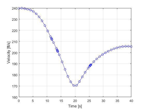
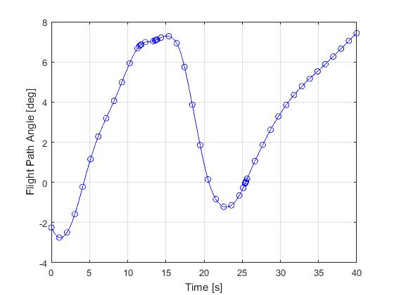
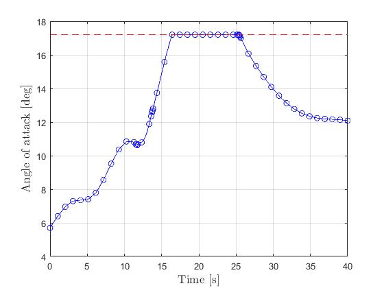
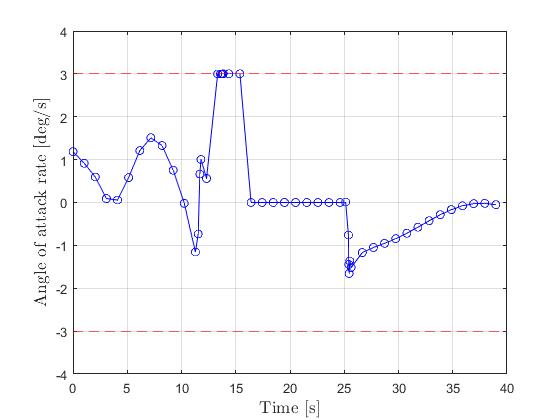
Results from ICLOCS2
Using the 'AutoDirect' (Automatic chosen direct collocation) method of ICLOCS2, the following state and input trajectories are obtained after 6 mesh refinement iterations starting from 40 equally spaced mesh points with the Hermite-Simpson discretization scheme.
The total computation time is about 7 seconds using finite difference derivative calculations on an Intel i7-6700 desktop computer. Subsequent recomputation using the refined mesh and warm starting will take on average 1 seconds and 22 iterations.
It is interesting to note that if equally spaced mesh was to be used without mesh refinement, then approximately 900 points are needed to fulfill the error tolerance requirements. In that case, the computation time will increase to 20 seconds (186% higher) and subsequent recomputation using the same mesh and warm starting will take on average 13 seconds (1300% higher). This clearly demonstrated the benefit and necessity of mesh refinement .
[1] R. Bulirsch, F. Montrone, and H. Pesch, Abort landing in the presence of windshear as a minimax optimal control problem, part 1: Necessary conditions, Journal of Optimization Theory and Applications, 70(1), pp 1-23, 1991.
[2] R. Bulirsch, F. Montrone, and H. Pesch, Abort landing in the presence of windshear as a minimax optimal control problem, part 2: Multiple shooting and homotopy, Journal of Optimization Theory and Applications, 70(2), pp 223-254, 1991.
[3] J. Betts, Practical Methods for Optimal Control and Estimation Using Nonlinear Programming: Second Edition, Advances in Design and Control, Society for Industrial and Applied Mathematics, 2010.