Example: Bang-bang Control (Multi-Phase)
Difficulty: Intermediate
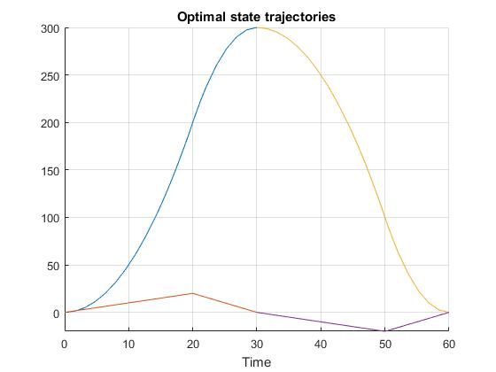
This problem is an extention to the single phase bang-bang control problem. Now, we would like to have the double integrator system to be repositioned from x=0 [m] to x=300 [m] and then back to x=0 [m] in mimimum time.
Formulate the problem in ICLOCS2
Problem definition for multiphase problem
In problem defination file BangBang.m, we can define the time variables for different phases
problem.mp.time.t_min=[0 0 0];
problem.mp.time.t_max=[0 70 70];
guess.mp.time=[0 30 60];
the static parameters (as part of optimization variables)
problem.mp.parameters.pl=[];
problem.mp.parameters.pu=[];
guess.mp.parameters=[];
and the lower bound, uppder bound and tolerance for some linear and nonlinear linkage constraints.
problem.mp.constraints.bll.linear=[0 0];
problem.mp.constraints.blu.linear=[0 0];
problem.mp.constraints.blTol.linear=[0.01 0.01];

problem.mp.constraints.bll.nonlinear=[];
problem.mp.constraints.blu.nonlinear=[];
problem.mp.constraints.blTol.nonlinear=[];
Next, we need to specify different phases of the OCP as well as the corresponding settings for each phase
[problem.phases{1},guess.phases{1}] = BangBangTwoPhase_Phase1(problem.mp, guess.mp);
[problem.phases{2},guess.phases{2}] = BangBangTwoPhase_Phase2(problem.mp, guess.mp);
phaseoptions{1}=problem.phases{1}.settings(20);
phaseoptions{2}=problem.phases{2}.settings(20);
In the linkage constraint function bclink, we can define the linkage constraint equations as
blc_linear=[xf{1}(1)-x0{2}(1);xf{1}(2)-x0{2}(2)];
blc_nonlinear=[];Problem definition for individual phases
First, the problem definition for the individual phases can be specified following the same guideline as for single-phase problems. For this particular example, we generated the following files
- BangBang_Dynamics_Phase1.m: same as BangBang_Dynamics_Internal.m
- BangBangTwoPhase_Phase1.m: same as BangBang.m, with minor differences. The main ones are for the time variables
for static parameters,
% Initial time.
problem.time.t0_idx=1;
problem.time.t0_min=problem_mp.time.t_min(problem.time.t0_idx);
problem.time.t0_max=problem_mp.time.t_max(problem.time.t0_idx);
guess.t0=guess_mp.time(problem.time.t0_idx);

% Final time. Let tf_min=tf_max if tf is fixed.
problem.time.tf_idx=2;
problem.time.tf_min=problem_mp.time.t_min(problem.time.tf_idx);
problem.time.tf_max=problem_mp.time.t_max(problem.time.tf_idx);
guess.tf=guess_mp.time(problem.time.tf_idx);
for the data storage static parameters% Parameters bounds. problem.parameters.pl=problem_mp.parameters.pl; problem.parameters.pu=problem_mp.parameters.pu; guess.parameters=guess_mp.parameters;and in the Mayer cost function E_unscaledproblem.data=problem_mp.data;boundaryCost=0; - BangBangTwoPhase_Phase2.m: same as BangBang.m, with minor differences. The main ones are for the time variables
for static parameters,
% Initial time.
problem.time.t0_idx=2;
problem.time.t0_min=problem_mp.time.t_min(problem.time.t0_idx);
problem.time.t0_max=problem_mp.time.t_max(problem.time.t0_idx);
guess.t0=guess_mp.time(problem.time.t0_idx);

% Final time. Let tf_min=tf_max if tf is fixed.
problem.time.tf_idx=3;
problem.time.tf_min=problem_mp.time.t_min(problem.time.tf_idx);
problem.time.tf_max=problem_mp.time.t_max(problem.time.tf_idx);
guess.tf=guess_mp.time(problem.time.tf_idx);
for state variables,% Parameters bounds. problem.parameters.pl=problem_mp.parameters.pl; problem.parameters.pu=problem_mp.parameters.pu; guess.parameters=guess_mp.parameters;for input variable,% Initial conditions for system. problem.states.x0l=[0 -200]; problem.states.x0u=[300 200]; % State bounds problem.states.xl=[0 -200]; problem.states.xu=[310 200]; % Terminal state bounds. problem.states.xfl=[0 0]; problem.states.xfu=[0 0]; % Guess the state trajectories with [x0 xf] guess.states(:,1)=[100 0]; guess.states(:,2)=[-50 0];and for the data storage static parameters% Input bounds problem.inputs.ul=[-1]; problem.inputs.uu=[2]; % Bounds on first control action problem.inputs.u0l=[-1]; problem.inputs.u0u=[2]; % Guess the input sequences with [u0 uf] guess.inputs(:,1)=[-1 2];problem.data=problem_mp.data; - gradCost_BangBang_Phase1.m: same as gradCost_BangBang.m
- gradCost_BangBang_Phase2.m: same as gradCost_BangBang.m
- hessianLagrangian_BangBang.m: same as hessianLagrangian_BangBang.m
- jacConst_BangBang.m: same as jacConst_BangBang.m
- settings_BangbangTwoPhase_Phase1.m: same as settings_Bangbang.m, but only contains phase depended settings
- settings_BangbangTwoPhase_Phase2.m: same as settings_Bangbang.m, but only contains phase depended settings
Main script main_BangbangTwoPhase.m for solving the multi-phase bang-bang control problem
Now we can fetch the problem and options, solve the resultant NLP, and generate some plots for the solution.
[problem,guess,options.phaseoptions]=BangBangTwoPhase; % Fetch the problem definition
options.mp= settings_BangbangTwoPhase; % Get options and solver settings
[solution,MRHistory]=solveMyProblem( problem,guess,options);
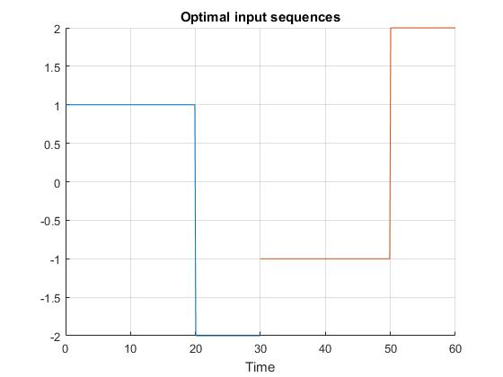
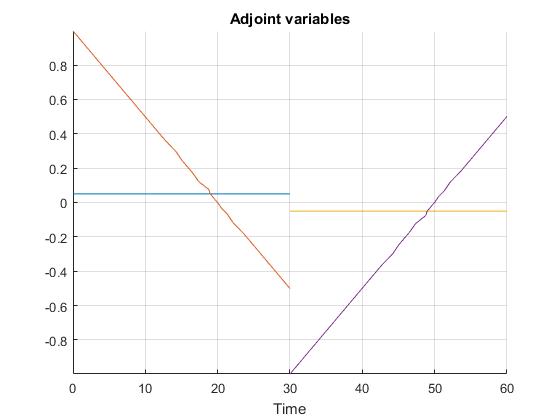
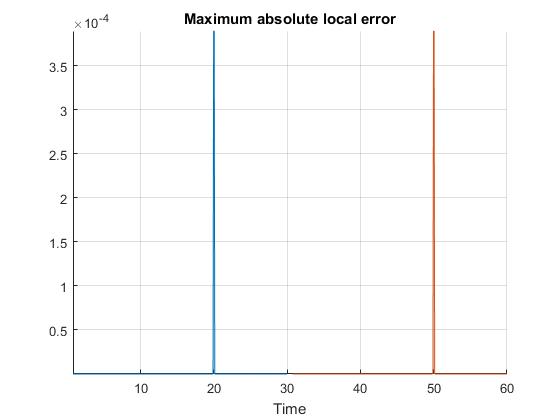
genSolutionPlots(options, solution);Results from ICLOCS2
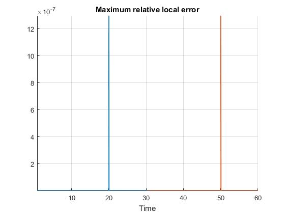
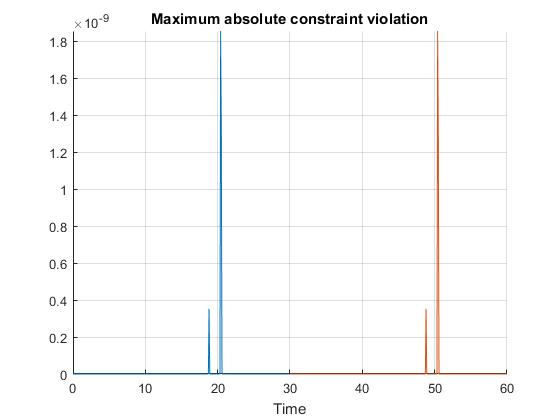
Using the Hermite-Simpson discretization scheme of ICLOCS2, the following state and input trajectories are obtained under a mesh refinement scheme starting with 20 mesh points for each phase. The computation time with IPOPT (NLP convergence tol set to 1e-09) is about 1 seconds with one mesh refinement iteration altogether, using analytical derivative calculations on an Intel i7-6700 desktop computer. The graphs are generated by ICLOCS 2.5 built-in genSolutionPlots command.