Example
Minimum Time Flight Profile for a Commercial Aircraft
Difficulty: Hard
The aerodynamic and propulsion data are obtained from [1].
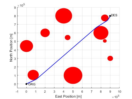
Consider the flight mission of a commerical aircraft illustrated below
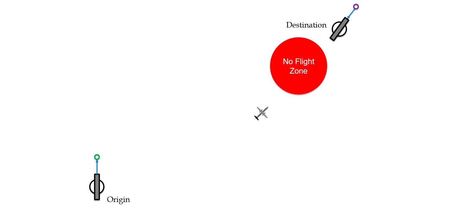
The objective is find the optimal control profile such that the aircraft reach the destination in shortest time:

subject to dynamic constraints
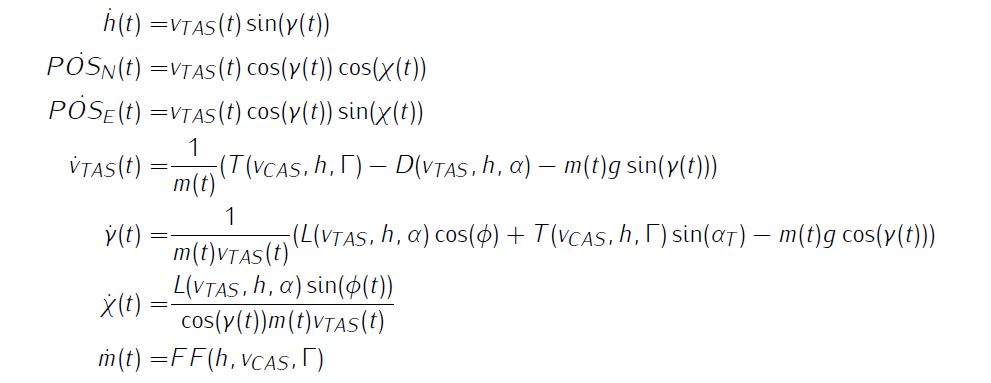
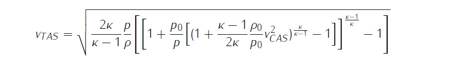
with the airspeed conversion as
For this scenario, we have path constraint for avoiding a number of no flight zone (NFZ)

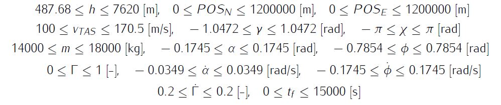
Additionally, there are simple bounds on variables,
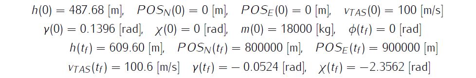
and boundary conditions
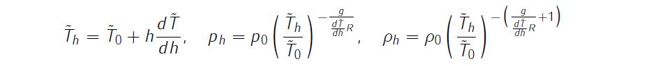
Details about the aerodynamic and propulsion modelling are available in the reference, thus will not be reproduced here. For this problem, a simple atmospheric model is used
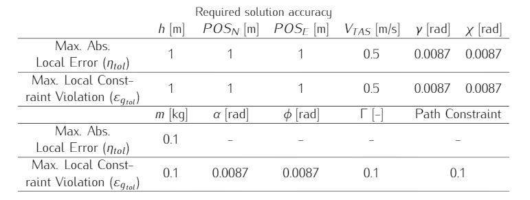
We require the numerical solution to fulfill the following accuracy criteria
Formulate the problem in ICLOCS2
In internal model defination file CommericalFlightProfile_Dynamics_Internal.m
We can specify the system dynamics in function CommericalFlightProfile_Dynamics_Internal with
auxdata = data.auxdata;

H = x(:,1);
npos = x(:,2);
epos = x(:,3);
V_tas = x(:,4);
gamma = x(:,5);
chi = x(:,6);
W = x(:,7);
alpha = u(:,1);
phi = u(:,2);
throttle = u(:,3);

Temp=auxdata.Ts+H*auxdata.dTdH;
pressure=auxdata.ps*(Temp./auxdata.Ts).^(-auxdata.g/auxdata.dTdH/auxdata.R);
rho=auxdata.rhos*(Temp./auxdata.Ts).^(-(auxdata.g/auxdata.dTdH/auxdata.R+1));
[ V_cas ] = CAS2TAS( auxdata.kappa, pressure, rho, auxdata.ps, auxdata.rhos, V_tas );

ap=auxdata.a1p.*V_cas.^2+auxdata.a2p.*V_cas+auxdata.a3p;
bp=auxdata.b1p.*V_cas.^2+auxdata.b2p.*V_cas+auxdata.b3p;
cp=auxdata.c1p.*V_cas.^2+auxdata.c2p.*V_cas+auxdata.c3p;
Pmax=ap.*H.^2+bp.*H+cp;

P=(Pmax-auxdata.Pidle).*throttle+auxdata.Pidle;
J=60*V_tas/auxdata.nprop/auxdata.Dprop;
ita=-0.13289*J.^6+1.2536*J.^5-4.8906*J.^4+10.146*J.^3-11.918*J.^2+7.6740*J-1.3452;
Thrust=2*745.6*ita.*P./V_tas;

% Calculate aerodynamic forces
cl=auxdata.clalpha.*(alpha-auxdata.alpha0)*180/pi;
L=0.5.*cl.*rho.*V_tas.^2.*auxdata.S;
cd=auxdata.cd0+auxdata.k_cd*cl.^2;
Drag=0.5.*cd.*rho.*V_tas.^2.*auxdata.S;

%% equations of motions
TAS_dot=(Thrust-Drag-W.*sin(gamma)).*auxdata.g./W;
gamma_dot=(L.*cos(phi)+Thrust*sin(auxdata.alphat)-W.*cos(gamma))*auxdata.g./W./V_tas;
H_dot=V_tas.*sin(gamma);
x_dot=V_tas.*cos(gamma).*cos(chi);
y_dot=V_tas.*cos(gamma).*sin(chi);
chi_dot=L.*sin(phi)./cos(gamma)*auxdata.g./W./V_tas;
W_dot= calcWeight(V_cas,H,throttle,auxdata.FFModel);

c1=(npos-data.auxdata.obs_npos_1).^2+(epos-data.auxdata.obs_epos_1).^2-data.auxdata.obs_r_1.^2;
c2=(npos-data.auxdata.obs_npos_2).^2+(epos-data.auxdata.obs_epos_2).^2-data.auxdata.obs_r_2.^2;
c3=(npos-data.auxdata.obs_npos_3).^2+(epos-data.auxdata.obs_epos_3).^2-data.auxdata.obs_r_3.^2;
c4=(npos-data.auxdata.obs_npos_4).^2+(epos-data.auxdata.obs_epos_4).^2-data.auxdata.obs_r_4.^2;
c5=(npos-data.auxdata.obs_npos_5).^2+(epos-data.auxdata.obs_epos_5).^2-data.auxdata.obs_r_5.^2;
c6=(npos-data.auxdata.obs_npos_6).^2+(epos-data.auxdata.obs_epos_6).^2-data.auxdata.obs_r_6.^2;
c7=(npos-data.auxdata.obs_npos_7).^2+(epos-data.auxdata.obs_epos_7).^2-data.auxdata.obs_r_7.^2;
c8=(npos-data.auxdata.obs_npos_8).^2+(epos-data.auxdata.obs_epos_8).^2-data.auxdata.obs_r_8.^2;
c9=(npos-data.auxdata.obs_npos_9).^2+(epos-data.auxdata.obs_epos_9).^2-data.auxdata.obs_r_9.^2;
c10=(npos-data.auxdata.obs_npos_10).^2+(epos-data.auxdata.obs_epos_10).^2-data.auxdata.obs_r_10.^2;

%%
dx = [H_dot, x_dot, y_dot, TAS_dot, gamma_dot, chi_dot, W_dot];
g_neq=[c1,c2,c3,c4,c5,c6,c7,c8,c9,c10]/1e04;
For this example problem, we have several inequality path constraints, so function CommericalFlightProfile_Dynamics_Internal need to return the value of variable dx and g_neq . Also note that the Heaviside functions are approximated with tanh functions for differentiability.
Similarly, the (optional) simulation dynamics can be specifed in function CommericalFlightProfile.m .
In problem defination file CommericalFlightProfile.m
First we provide the function handles for system dynamics with
InternalDynamics=@CommericalFlightProfile_Dynamics_Internal;
SimDynamics=@CommericalFlightProfile_Dynamics_Sim;
The optional files providing analytic derivatives can be left empty as we use of finite difference this time
problem.analyticDeriv.gradCost=[];
problem.analyticDeriv.hessianLagrangian=[];
problem.analyticDeriv.jacConst=[];
and finally the function handle for the settings file is given as.
problem.settings=@settings_CommericalFlightProfile;Next we define the parameters for the scenario,
% Thrust model
x=[0 0.5 1];
y=[0 0.48 1];
FFModel=pchip(x,y);

% Constants
auxdata.g=9.81;
auxdata.ktomps=0.514444;
auxdata.ftom=0.3048;
auxdata.R=287.15;
auxdata.ps=101325;
auxdata.rhos=1.225;
auxdata.Ts=288.15;
auxdata.dTdH=-0.0065;
auxdata.nprop=1020;
auxdata.Dprop=3.66;
auxdata.kappa=1.4;
auxdata.alpha0=-2.32*pi/180;
auxdata.clalpha=0.095;
auxdata.k_cd=0.033;
auxdata.cd0=0.0233;
auxdata.S=70;
auxdata.alphat=0*pi/180;
auxdata.FFModel=FFModel;

% Look up tables
auxdata.a1p=1.5456*10^-9;
auxdata.a2p=-3.1176*10^-7;
auxdata.a3p=1.9477*10^-5;
auxdata.b1p=-2.0930*10^-5;
auxdata.b2p=4.1670*10^-3;
auxdata.b3p=-0.40739;
auxdata.c1p=0.088835;
auxdata.c2p=-12.855;
auxdata.c3p=3077.7;
auxdata.Pidle=75;
and declear the variables for later use.
% initial conditions
W0=18000*auxdata.g;
H0=1600*auxdata.ftom;
T0=auxdata.Ts+H0*auxdata.dTdH;
p0=auxdata.ps*(T0/auxdata.Ts)^(-auxdata.g/auxdata.dTdH/auxdata.R);
rho0=auxdata.rhos*(T0/auxdata.Ts)^(-(auxdata.g/auxdata.dTdH/auxdata.R+1));
Vtas0=CAS2TAS( auxdata.kappa, p0, rho0, auxdata.ps, auxdata.rhos, 190*auxdata.ktomps );
x0=0;y0=0;
alpha0=5*pi/180;
chi0=0;
gamma0=8*pi/180;

% variable bounds
W_min=(18000-4000)*auxdata.g;
H_min=H0;H_max=25000*auxdata.ftom;
T_Hmax=auxdata.Ts+H_max*auxdata.dTdH;
p_Hmax=auxdata.ps*(T_Hmax/auxdata.Ts)^(-auxdata.g/auxdata.dTdH/auxdata.R);
rho_Hmax=auxdata.rhos*(T_Hmax/auxdata.Ts)^(-(auxdata.g/auxdata.dTdH/auxdata.R+1));
Vtas_max=CAS2TAS( auxdata.kappa, p_Hmax, rho_Hmax, auxdata.ps, auxdata.rhos, 227*auxdata.ktomps );
Vtas_min=Vtas0;
alpha_max=10*pi/180;
gamma_max=60*pi/180;
throttle_max=1;throttle_min=0;
chi_max=pi;
chi_min=-pi;
phi_0=0;
phi_max=45*pi/180;
x_max=1200000;
y_max=1200000;

% terminal conditions
Hf=2000*auxdata.ftom;
T_Hf=auxdata.Ts+Hf*auxdata.dTdH;
p_Hf=auxdata.ps*(T_Hf/auxdata.Ts)^(-auxdata.g/auxdata.dTdH/auxdata.R);
rho_Hf=auxdata.rhos*(T_Hf/auxdata.Ts)^(-(auxdata.g/auxdata.dTdH/auxdata.R+1));
Vtasf=CAS2TAS( auxdata.kappa, p_Hf, rho_Hf, auxdata.ps, auxdata.rhos, 190*auxdata.ktomps );
xf=800000;
yf=900000;
chif=-3/4*pi;
gammaf=-3*pi/180;

% Parameter for the obstacle
auxdata.obs_npos_1=775000;
auxdata.obs_epos_1=842000;
auxdata.obs_r_1=40000;

auxdata.obs_npos_2=545000;
auxdata.obs_epos_2=442000;
auxdata.obs_r_2=30000;

auxdata.obs_npos_3=505000;
auxdata.obs_epos_3=842000;
auxdata.obs_r_3=20000;


auxdata.obs_npos_4=105000;
auxdata.obs_epos_4=72000;
auxdata.obs_r_4=60000;

auxdata.obs_npos_5=445000;
auxdata.obs_epos_5=0;
auxdata.obs_r_5=70000;

auxdata.obs_npos_6=600000;
auxdata.obs_epos_6=200000;
auxdata.obs_r_6=50000;

auxdata.obs_npos_7=100000;
auxdata.obs_epos_7=500000;
auxdata.obs_r_7=100000;

auxdata.obs_npos_8=300000;
auxdata.obs_epos_8=300000;
auxdata.obs_r_8=60000;

auxdata.obs_npos_8=800000;
auxdata.obs_epos_8=400000;
auxdata.obs_r_8=90000;

auxdata.obs_npos_9=300000;
auxdata.obs_epos_9=900000;
auxdata.obs_r_9=30000;


auxdata.obs_npos_10=600000;
auxdata.obs_epos_10=800000;
auxdata.obs_r_10=80000;
Now we may define the time variables with
problem.time.t0_min=0;
problem.time.t0_max=0;
guess.t0=0;
and
problem.time.tf_min=7000;
problem.time.tf_max=10000;
guess.tf=8500;
For state variables, we need to provide the initial conditions
problem.states.x0=[H0 x0 y0 Vtas0 gamma0 chi0 W0]; bounds on intial conditions
problem.states.x0l=[H0 x0 y0 Vtas0 gamma0 chi0 W0];
problem.states.x0u=[H0 x0 y0 Vtas0 gamma0 chi0 W0];
state bounds
problem.states.xl=[H_min x0 y0 Vtas_min -gamma_max chi_min W_min];
problem.states.xu=[H_max x_max y_max Vtas_max gamma_max chi_max W0];
state rate bounds
problem.states.xrl=[-inf -inf -inf -inf -inf -inf -inf];
problem.states.xru=[inf inf inf inf inf inf inf];
bounds on the absolute local and global (integrated) discretization error of state variables
problem.states.xErrorTol_local=[1 1 1 0.5 deg2rad(5) deg2rad(5) 0.1*auxdata.g];
problem.states.xErrorTol_integral=[1 1 1 0.5 deg2rad(5) deg2rad(5) 0.1*auxdata.g];
tolerance for state variable and state rate box constraint violation
problem.states.xConstraintTol=[1 1 1 0.5 deg2rad(5) deg2rad(5) 0.1*auxdata.g];
problem.states.xrConstraintTol=[1 1 1 0.5 deg2rad(5) deg2rad(5) 0.1*auxdata.g];
terminal state bounds
problem.states.xfl=[Hf xf yf Vtasf gammaf chif W_min];
problem.states.xfu=[Hf xf yf Vtasf gammaf chif W0];
and an initial guess of the state trajectory (optional but recommended)
guess.states(:,1)=[H_max H_max];
guess.states(:,2)=[x0 xf];
guess.states(:,3)=[y0 yf];
guess.states(:,4)=[Vtas_max Vtas_max];
guess.states(:,5)=[gamma0 gammaf];
guess.states(:,6)=[chi0 chif];
guess.states(:,7)=[W0 (18000-2000)*auxdata.g];
Lastly for control variables, we need to define simple bounds
problem.inputs.ul=[-alpha_max -phi_max throttle_min];
problem.inputs.uu=[alpha_max phi_max throttle_max];
bounds on the first control action
problem.inputs.u0l=[-alpha_max -phi_max throttle_min];
problem.inputs.u0u=[alpha_max phi_max throttle_max];
control input rate constraint
problem.inputs.url=[-deg2rad(2) -deg2rad(10) -0.2];
problem.inputs.uru=[deg2rad(2) deg2rad(10) 0.2];
tolerance for control variable box constraint and rate constraint violations
problem.inputs.uConstraintTol=[deg2rad(0.5) deg2rad(0.5) 0.1];
problem.inputs.urConstraintTol=[deg2rad(0.5) deg2rad(0.5) 0.1];
as well as initial guess of the input trajectory (optional but recommended)
guess.inputs(:,1)=[alpha0 alpha0];
guess.inputs(:,2)=[phi_0 phi_0];
guess.inputs(:,3)=[1 1];
Additionally, we need to specify the bounds for the constraint functions . We have no equality path constraint
problem.constraints.ng_eq=0;
problem.constraints.gTol_eq=[];
but do have a number of inequality path constraint
problem.constraints.gl=[0 0 0 0 0 0 0 0 0 0];
problem.constraints.gu=[inf inf inf inf inf inf inf inf inf inf];
problem.constraints.gTol_neq=[(auxdata.obs_r_1+5)^2-(auxdata.obs_r_1)^2 (auxdata.obs_r_2+5)^2-(auxdata.obs_r_2)^2 (auxdata.obs_r_3+5)^2-(auxdata.obs_r_3)^2 (auxdata.obs_r_4+5)^2-(auxdata.obs_r_4)^2 (auxdata.obs_r_5+5)^2-(auxdata.obs_r_5)^2 (auxdata.obs_r_6+5)^2-(auxdata.obs_r_6)^2 (auxdata.obs_r_7+5)^2-(auxdata.obs_r_7)^2 (auxdata.obs_r_8+5)^2-(auxdata.obs_r_8)^2 (auxdata.obs_r_9+5)^2-(auxdata.obs_r_9)^2 (auxdata.obs_r_10+5)^2-(auxdata.obs_r_10)^2]/1e04;
and boundary constraint function
problem.constraints.bl=[0];
problem.constraints.bu=[0];
problem.constraints.bTol=[0.1];
We may store the necessary problem parameters used in the functions
problem.data.auxdata=auxdata;Since this problem only has a Mayer (boundary) cost , and no Lagrange (stage) cost ,we simply have
boundaryCost=tf;stageCost = 0*t;for sub-function E_unscaled and L_unscaled respectively.
Sub-routine b_unscaled for boundary constraints will need to be defined as
bc=[uf(2)];Main script main_CommericalFlightProfile.m
Now we can fetch the problem and options, solve the resultant NLP, and generate some plots for the solution.
[problem,guess]=CommericalFlightProfile;          % Fetch the problem definition
options= problem.settings(60);                  % Get options and solver settings
[solution,MRHistory]=solveMyProblem( problem,guess,options);
Results from ICLOCS2
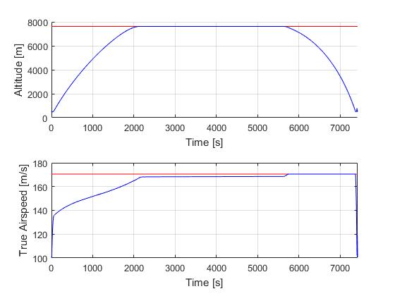
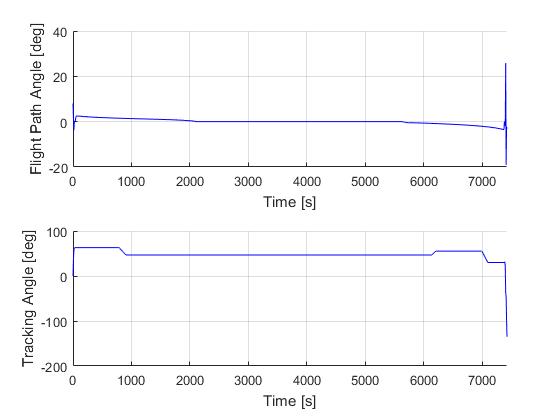
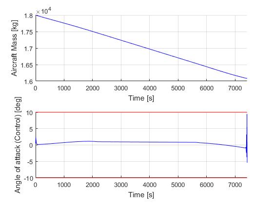
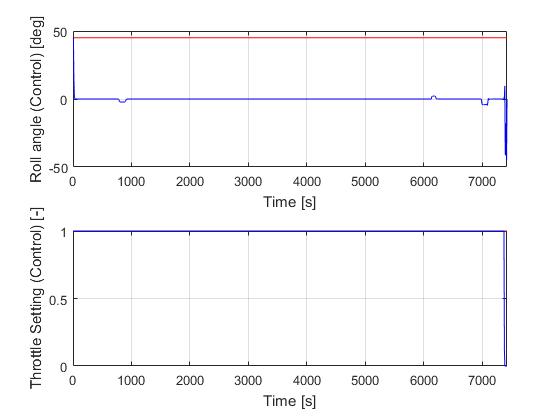
Using the Hermite-Simpson discretization scheme of ICLOCS2, the following state and input trajectories are obtained under a mesh refinement scheme starting with 60 mesh points.

The total computation time with IPOPT (NLP convergence tol set to 1e-07) is about 265 seconds (4.4 minutes) with 3 mesh refinement iterations altogether, using finite difference derivative calculations on an Intel i7-6700 desktop computer. Subsequent recomputation using the refined mesh and warm starting will take on average 40 seconds and 70 iterations. However it is important to note that the results are obtained with very rough initial guess, strict tolerance on discretization and constraint violation errors, and a flight of a relatively long duration (more than 2 hours).
In ICLOCS version 2.5, we have introduced an external constraint handling (ECH) scheme that can actively remove inactive constraints from the problem formulation. See HERE for more information. With ECH enabled, the computational time can be reduced to 166 seconds (2.7 minutes, 37% lower).
The final mesh contains 238 mesh intervals. If equally spaced mesh is used, even with 800 mesh points, the resultant errors are still significantly larger than that of the requirement. However, such a computation will already increase than 200%. This clearly demonstrated the benefit and necessity of mesh refinement .
[1] Performance model Fokker 50, Delft University of Technology, 2010