Example: Cart Pole Swing-Up Problem
Difficulty: Easy
This problem was originally presented in Section 6 of [1]. This example is available via the link on the right.
The implementation of this examples will not be explained in details due to similarity with other examples. Please refer to an example with similar complexity for implementation instructions, or other examples in the list of examples with Detailed Instructions.
Results from ICLOCS2: Trajectory Optimization
Using the Hermite-Simpson discretization scheme of ICLOCS2, the following state and input trajectories are obtained under a mesh refinement scheme starting with 30 mesh points. The computation time with IPOPT (NLP convergence tol set to 1e-09) is about 1 seconds for 3 mesh refinement iterations together, using analytical derivative calculations on an Intel i7-6700 desktop computer. Subsequent recomputation using the same mesh and warm starting will take on average 0.3 seconds and about 10 iterations.
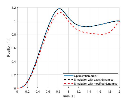
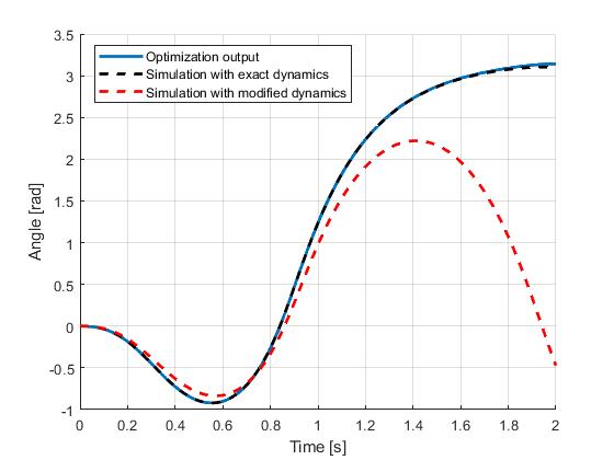
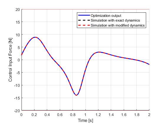
Seen in the figures, although the open-loop simulation using the model with exact same dynamics only yield minor differences, the red dashlines indicate that under a moderate parameter uncertainty (pole length: 0.5m => 0.55m, cart mass: 1kg => 1.1kg, pole mass: 0.3 => 0.28kg), the original input trajectory would fail to bring the pendulum into the inverted position.
Therefore, for such problems that are sensitive to uncertainties, closed-loop implementation of the optimial control solution would be required. Such implementation can be prototyped directly in ICLOCS2.5 with the Simulink interface.
Closed-loop Simulation
The closed-loop implementation of the optimial control solution can be done in a number of different ways. The most common approach would be to design a regulation typed (tracking) controller that would track the state trajectores of the optimial control solution. In the form of model predictive control (MPC), this would be realized with a quadratic regulation objective.
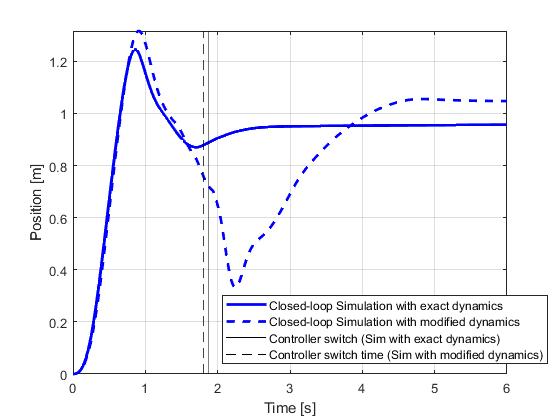
For this example, we will take a different approach to implement a two-phase control strategy. The first phase will try to exactly reproduce the original optimal control problem, however several modifications are needed as a preparation step. First point to notice is that without formulating the problem into a tracking problem, the popular receding horizon control strategy for MPC will not be directly suitable. The original problem has a fixed terminal-time of 2 seconds, with the movement of cart and invertion of pendulum imposed only at the terminal condition. Therefore, even without any uncertainties, the solution of subsequent optimization solves at later steps will only corresponds to the original solution if the fixed terminal time is being reduced accordingly in a shrinking horizon strategy.
With the shrinking horizon strategy, special attention needs to be paid to recursive feasiblity of the optimal control problem, when the implementation is subject to uncertainties such as plant-model mismatch and external disturbances. With these conditions, the terminal constraints may not be fulfillable under a short horizon leading to unsuccessful optimization. A possible solution to this problem demonstrated in this example is to implement the terminal conditions as soft constraints, and to introduce a lower bound on the terminal time to avoid numerical issuses with very small time duration (tf-t0 ≈ 0s).
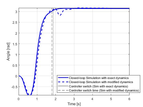
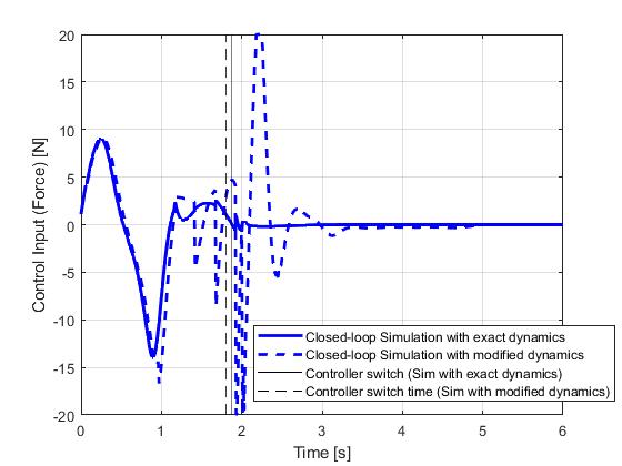
With the lower bound on the terminal time, the updated optimal control solution will deviate from the original solution near the end of the phase 1. This, however, will not be an issue practically as once the pendulum is almost inverted (+/- 5deg differences), the system will switch to the second phase controller aiming at maintaining the pendulum and the cart within a certain performance range (+/- 1deg for angle and +/- 0.1m for position, implemented as soft constraints) using minimum control effort (as objective). Unlike conventional quadratic regulation objective formulation which leads to trade-off between tracking performance and control effort at all times, this implementation has the benefit to solely reduce control effort when variables are within performance bounds. But if the performance degraded beyond the limit due to uncertainties, the controller will dedicate itself to quickly eliminate all constraint violations.
This example has already been implemented for you. You may use the Link to download it directly and feel free to use it as a starting point to formulate your own closed-loop simulations.
Results from ICLOCS2
The closed-loop simulation results are illustrated below with a simulation and re-optimization step of 0.01s. It can be seen that in spite of the model mismatches, the objectives of the cart pole swing-up problem have been successfully achieved.
Therefore, for such problems that are sensitive to uncertainties, closed-loop implementation of the optimial control solution would be required. Such implementation can be prototyped directly in ICLOCS2.5 with the Simulink interface.
[1] Kelly M. An introduction to trajectory optimization: How to do your own direct collocation. SIAM Review. 2017 Nov 6;59(4):849-904.