Example: Two Link Robot Arm
Difficulty: Easy
The problem was adapted from Example 2, Section 12.4.2 of [1].
Consider the system illustrated below
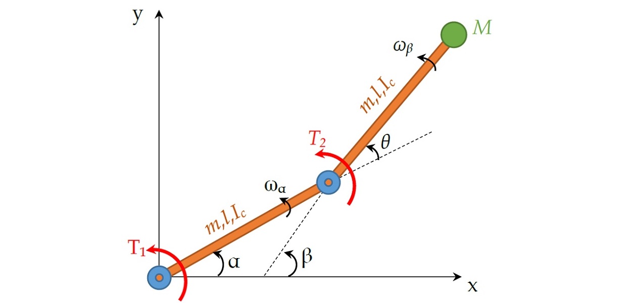
consisting of two identical beams with the same property (mass, length and moment of inerita), connected at two actuated joints. The objective is to formulate an optimal control problem to reposition the payload M using minimum time:

With the following assumptions and nondimensionalizations,
the system dynamics can then be expressed as
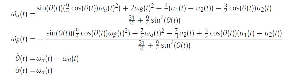
Additionally, we need simple bounds on variables

and boundary conditions

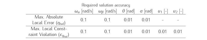
We require the numerical solution to fulfill the following accuracy criteria
Formulate the problem in ICLOCS2
In internal model defination file TwoLinkRobotArm_Dynamics_Internal.m
We can specify the system dynamics in function TwoLinkRobotArm_Dynamics_Internal with
x1 = x(:,1);x2 = x(:,2);x3 = x(:,3);
u1 = u(:,1);u2 = u(:,2);

dx(:,1) = (sin(x3).*(9/4*cos(x3).*x1.^2)+2*x2.^2 + 4/3*(u1-u2) - 3/2*cos(x3).*u2 )./ (31/36 + 9/4*sin(x3).^2);
dx(:,2) = -( sin(x3).*(9/4*cos(x3).*x2.^2)+7/2*x1.^2 - 7/3*u2 + 3/2*cos(x3).*(u1-u2) )./ (31/36 + 9/4*sin(x3).^2);
dx(:,3) = x2-x1;
dx(:,4) = x1;
For this example problem, we do not have any path constraints, so function TwoLinkRobotArm_Dynamics_Internal only need to return the value of variable dx .
Similarly, the (optional) simulation dynamics can be specifed in function TwoLinkRobotArm_Dynamics_Sim .
In problem defination file TwoLinkRobotArm.m
First we provide the function handles for system dynamics with,
InternalDynamics=@TwoLinkRobotArm_Dynamics_Internal;
SimDynamics=@TwoLinkRobotArm_Dynamics_Sim;
the optional files providing analytic derivatives can be left empty as we use finite difference this time
problem.analyticDeriv.gradCost=[];
problem.analyticDeriv.hessianLagrangian=[];
problem.analyticDeriv.jacConst=[];
and the function handle for the settings file.
problem.settings=@settings_TwoLinkRobotArm;Next we define the time variables with
problem.time.t0_min=0;
problem.time.t0_max=0;
guess.t0=0;
and
problem.time.tf_min=0.1;
problem.time.tf_max=inf;
guess.tf=3.1;
For state variables, we need to provide the initial conditions
problem.states.x0=[0 0 0 0];bounds on intial conditions
problem.states.x0l=[0 0 0 0];
problem.states.x0u=[0 0 0 0];
state bounds
problem.states.xl=[-inf -inf -inf -inf];
problem.states.xu=[inf inf inf inf];
bounds on the absolute local and global (integrated) discretization error of state variables
problem.states.xErrorTol_local=[deg2rad(0.1) deg2rad(0.1) deg2rad(0.05) deg2rad(0.05)];
problem.states.xErrorTol_integral=[deg2rad(0.1) deg2rad(0.1) deg2rad(0.05) deg2rad(0.05)];
tolerance for state variable box constraint violation
problem.states.xConstraintTol=[deg2rad(0.1) deg2rad(0.1) deg2rad(0.05) deg2rad(0.05)]; terminal state bounds
problem.states.xfl=[0 0 0.5 0.522];
problem.states.xfu=[0 0 0.5 0.522];
and an initial guess of the state trajectory (optional but recommended)
guess.states(:,1)=[0.1 0];
guess.states(:,2)=[0.1 0];
guess.states(:,3)=[0 0.5];
guess.states(:,4)=[0 0.522];
Lastly for control variables, we need to define simple bounds
problem.inputs.ul=[-1 -1];
problem.inputs.uu=[1 1];
bounds on the first control action
problem.inputs.u0l=[-1 -1];
problem.inputs.u0u=[1 1];
tolerance for control variable box constraint violation
problem.inputs.uConstraintTol=[0.01 0.01]; as well as an initial guess of the input trajectory (optional but recommended)
guess.inputs(:,1)=[1 -1];
guess.inputs(:,2)=[1 -1];
This problem has both Lagrange (stage) cost and Mayer (boundary) cost , thus we specify
stageCost = 0.01*(u(:,1).*u(:,1)+u(:,2).*u(:,2));boundaryCost=tf;for sub-function L_unscaled and E_unscaled respectively.
For this example problem, we do not have additional boundary constraints (in addition to varialbe simple bounds). Thus we can leave sub-routine b_unscaled as it is.
Main script main_TwoLinkRobotArm.m
Now we can fetch the problem and options, solve the resultant NLP, and generate some plots for the solution.
[problem,guess]=TwoLinkRobotArm;          % Fetch the problem definition
options= problem.settings(20);                  % Get options and solver settings
[solution,MRHistory]=solveMyProblem( problem,guess,options);
[ tv, xv, uv ] = simulateSolution( problem, solution, 'ode113', 0.01 );
Note the last line of code will generate an open-loop simulation, applying the obtained input trajectory to the dynamics defined in TwoLinkRobotArm_Dynamics_Sim.m , using the Matlab builtin ode113 ODE solver with a step size of 0.01.
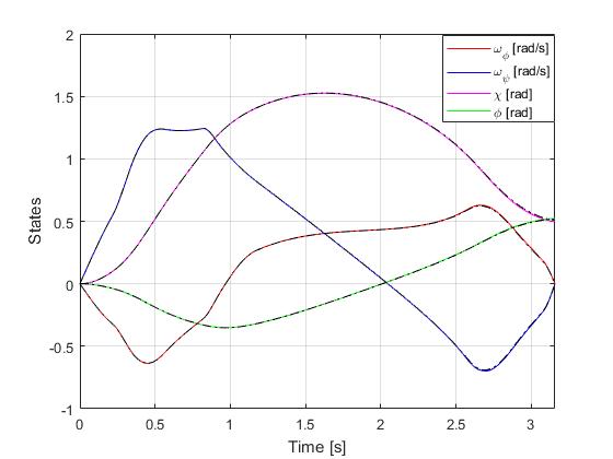
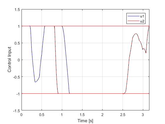
Results from ICLOCS2
Using the Hermite-Simpson discretization scheme of ICLOCS2, the following state and input trajectories are obtained under a mesh refinement scheme starting with 20 mesh points. The computation time with IPOPT (NLP convergence tol set to 1e-09) is about 2 seconds for 4 mesh refinement iterations together, using finite difference derivative calculations on an Intel i7-6700 desktop computer. Subsequent recomputation using the same mesh and warm starting will take on average 0.3 seconds and about 10 iterations.
[1] R. Luus, Iterative Dynamic Programming, Chapman and Hall/CRC Monographs and Surveys in Pure and Applied Mathematics, 2000.