Example: Batch Fermentor
Difficulty: Easy
The problem was originally presented by [1].
Consider the fed-batch reactor illustrated below
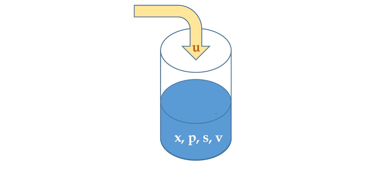
containing biomass (x), substrate (s) and product (p) at certain concentrations, and is of volume (v). The objective is find the optimal control profile for the substrate feed rate (u) such that the production is maximized:

The system dynamics can be expressed as
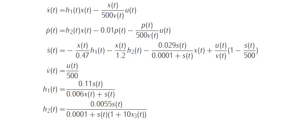
Additionally, we need simple bounds on variables

and boundary conditions

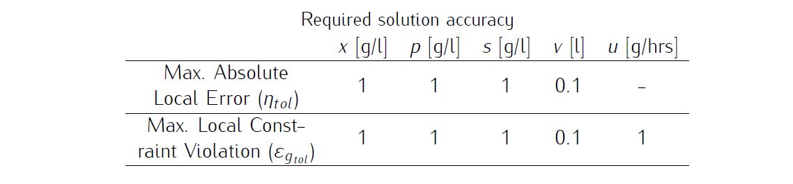
We require the numerical solution to fulfill the following accuracy criteria
Formulate the problem in ICLOCS2
In internal model defination file BatchFermentor_Dynamics_Internal.m
We can specify the system dynamics in function BatchFermentor_Dynamics_Internal with
x1 = x(:,1);x2 = x(:,2);x3 = x(:,3);x4 = x(:,4);
u1 = u(:,1);

h1 = 0.11*(x3./(0.006*x1+x3));
h2 = 0.0055*(x3./(0.0001+x3.*(1+10*x3)));

dx(:,1) = (h1.*x1-u1.*(x1./500./x4));
dx(:,2) = (h2.*x1-0.01*x2-u1.*(x2./500./x4));
dx(:,3) = (-h1.*x1/0.47-h2.*x1/1.2-x1.*(0.029*x3./(0.0001+x3))+u1./x4.*(1-x3/500));
dx(:,4) = u1/500;
For this example problem, we do not have any path constraints, so function BatchFermentor_Dynamics_Internal only need to return the value of variable dx .
Similarly, the (optional) simulation dynamics can be specifed in function BatchFermentor_Dynamics_Sim .
In problem defination file BatchFermentor.m
First we provide the function handles for system dynamics with,
InternalDynamics=@BatchFermentor_Dynamics_Internal;
SimDynamics=@BangBang_Dynamics_Sim;
the optional files providing analytic derivatives,
problem.analyticDeriv.gradCost=@gradCost_BatchFermentor;
problem.analyticDeriv.hessianLagrangian=@hessianLagrangian_BatchFermentor;
problem.analyticDeriv.jacConst=@jacConst_BatchFermentor;
and the function handle for the settings file.
problem.settings=@settings_BatchFermentor;Next we define the time variables with
problem.time.t0_min=0;
problem.time.t0_max=0;
guess.t0=0;
and
problem.time.tf_min=126;
problem.time.tf_max=126;
guess.tf=126;
For state variables, we need to provide the initial conditions
problem.states.x0=[1.5 0.0 0.0 7]; bounds on intial conditions
problem.states.x0l=[1.5 0.0 0.0 7];
problem.states.x0u=[40 50 25 10];
state bounds
problem.states.xl=[0 0 0 0];
problem.states.xu=[inf inf inf inf];
bbounds on the absolute local and global (integrated) discretization error of state variables
problem.states.xErrorTol_local=[0.1 0.1 0.1 0.1];
problem.states.xErrorTol_integral=[0.1 0.1 0.1 0.1];
tolerance for state variable box constraint violation
problem.states.xConstraintTol=[0.1 0.1 0.1 0.1]; terminal state bounds
problem.states.xfl=[0 0 0 0];
problem.states.xfu=[40 50 25 10];
and an initial guess of the state trajectory (optional but recommended)
guess.states(:,1)=[1.5 30];
guess.states(:,2)=[0 8.5];
guess.states(:,3)=[0 0];
guess.states(:,4)=[7 10];
Lastly for control variables, we need to define simple bounds
problem.inputs.ul=0;
problem.inputs.uu=50;
bounds on the first control action
problem.inputs.u0l=0;
problem.inputs.u0u=50;
tolerance for control variable box constraint violation
problem.inputs.uConstraintTol=0.1; as well as an initial guess of the input trajectory (optional but recommended)
guess.inputs(:,1)=[2 10];This problem has both Lagrange (stage) cost and Mayer (boundary) cost , thus we specify
stageCost =0.00001*u(:,1).*u(:,1);boundaryCost=-xf(2)*xf(4);for sub-function L_unscaled and E_unscaled respectively.
For this example problem, we do not have path constraints, variable rate constraints and additional boundary constraints (in addition to varialbe simple bounds). Thus we can leave sub-routines g_unscaled , avrc_unscaled and b_unscaled as they are.
Analytical derivatives
The analytical derivatives for the problem can be supplied with the following additional files: gradCost_BatchFermentor.m for cost gradient, jacConst_BatchFermentor.m for constraint Jacobian, and hessianLagrangian_BatchFermentor.m for the Lagrangian Hessian. Instructions on how to formulate these files are included in the function descriptions.
Main script main_BatchFermentor.m
Now we can fetch the problem and options, solve the resultant NLP, and generate some plots for the solution.
[problem,guess]=BatchFermentor;          % Fetch the problem definition
options= problem.settings(300);                  % Get options and solver settings
[solution,MRHistory]=solveMyProblem( problem,guess,options);
[ tv, xv, uv ] = simulateSolution( problem, solution, 'ode113', 0.01 );
Note the last line of code will generate an open-loop simulation, applying the obtained input trajectory to the dynamics defined in BatchFermentor_Dynamics_Sim.m , using the Matlab builtin ode113 ODE solver with a step size of 0.01.
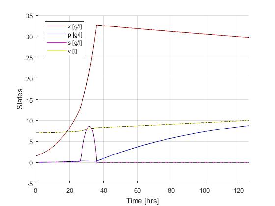
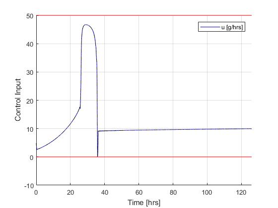
Results from ICLOCS2
With the existance of singular control in this problem, it is recommended to solve the problem using a realtively dense mesh instead of mesh refinement schemes. This is becasue the fluctuations and ringing phenomena on the singular arc are known to make mesh refinement process diverge. In this case, one often have to make large compromises between solution speed and result accuracy. Here, we focus on the accuracy of the solution.
Using the Hermite-Simpson discretization scheme of ICLOCS2, the following state and input trajectories are obtained using an uniform mesh with 299 intervals. The computation time with IPOPT (NLP convergence tol set to 1e-09) is about 20 seconds , using finite difference derivative calculations on an Intel i7-6700 desktop computer.
If analytical derivative infomations are supplied in ICLOCS2, the total computation time can be reduced to 3 seconds (reduction of 85%).
[1] J.E. Cuthrell and L. T. Biegler, Simultaneous optimization and solution methods for batch reactor control profiles, Computers and Chemical Engineering, 13:49-62, 1989.