ICLOCS2

This problem was presented as Example 4.9 of [1], with the challenge of being a singular control problem. This example is available via the link on the right.

The implementation of this examples will not be explained in details due to similarity with other examples. Please refer to an example with similar complexity for implementation instructions, or other examples in the list of examples with Detailed Instructions.

With the existance of singular control in this problem, it is recommended to solve the problem using a realtively dense mesh instead of mesh refinement schemes. This is becasue the fluctuations and ringing phenomena on the singular arc are known to make mesh refinement process diverge. In this case, one often have to make large compromises between solution speed and result accuracy. Here, we focus on the accuracy of the solution.

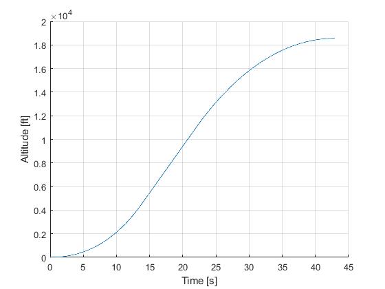
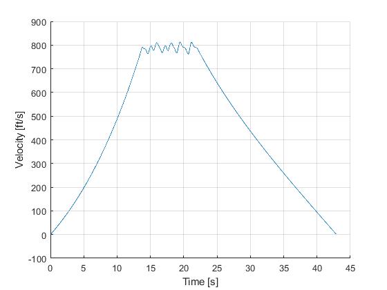
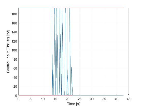
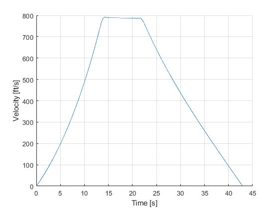
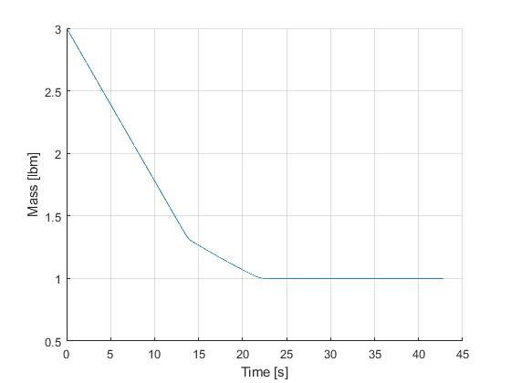
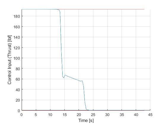
Using the Hermite-Simpson discretization scheme of ICLOCS2, the following state and input trajectories are obtained using an uniform mesh with 99 intervals, with direct collocation method and IPOPT (NLP convergence tol set to 1e-09). The influence of singular arc can still be clearly observed.

In this situation, the integrated residual minimization method of ICLOCS2 can be utilizaed, with the benefit to largly suppress the fluctuations in the solution caused by the singular arc. This can either be done at the solution representation level or as a standalone optimal control solution technique.

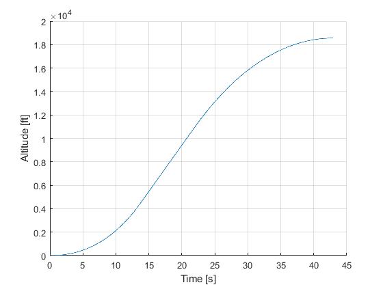
Wite the same Hermite-Simpson discretization scheme and uniform mesh with 99 intervals, the following state and input trajectories are obtained using the alternating varient of the integrated residual minimization method.

Since the singular arc exists distinctively for only one of the three phases of the flight, another alternative is to use a multi-phase formulation and specifify the singular arc conditions. We recommend this implementation as the most reliable approach.