Get Started
Formulate your problem in ICLOCS2: single phase problems
Formulating an optimal control problem in ICLOCS2 is straight-forward, and this guide will assist you in setting up the problem correctly and efficiently.
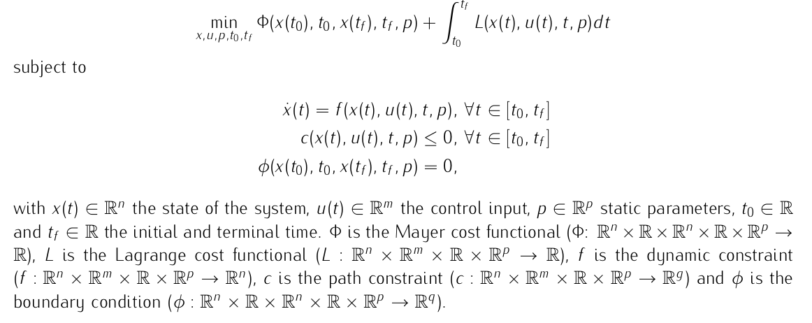
A general purpose optimal control problem can be formulated in the following Bolza form
and can be directly implement in ICLOCS2 through the following procedures.
In internal model defination file myProblem_Dynamics_Internal.m
We can specify the system dynamics and path constraints in function myProblem_Dynamics_Internal(x,u,p,t,vdat) with
%Obtain stored data
auxdata = vdat.auxdata;

%Define states
x1 = x(:,1);
%...
xn=x(:,n),

%Define inputs
u1 = u(:,1);
% ...
um = u(:,m);

%Define ODE right-hand side
dx(:,1) = f1(x1,..xn,u1,..um,p,t);
%...
dx(:,n) = fn(x1,..xn,u1,..um,p,t);

%Define path constraints (optional)
g_eq(:,1)=g_eq1(x1,...,u1,...p,t);
g_eq(:,2)=g_eq2(x1,...,u1,...p,t);

g_neq(:,1)=g_neq1(x1,...,u1,...p,t);
g_neq(:,2)=g_neq2(x1,...,u1,...p,t);
where the function myProblem_Dynamics_Internal returns the value of variable dx for system dynamics, and optionally g_eq for equality path constraints and g_neq for inequality constraints.
Similarly, the (optional) simulation dynamics can be specifed in function myProblem_Dynamics_Sim .
In problem defination file myProblem.m
Function Handles
First we provide the function handles for system dynamics with,
InternalDynamics=@myProblem_Dynamics_Internal;
SimDynamics=@myProblem_Dynamics_Sim;
the optional files providing analytic derivatives,
problem.analyticDeriv.gradCost=@gradCost;
problem.analyticDeriv.hessianLagrangian=@hessianLagrangian;
problem.analyticDeriv.jacConst=@jacConst;
and the function handle for the settings file.
problem.settings=@settings_myProblem;Time Variables
Next we define the time variables with
problem.time.t0_min=0;
problem.time.t0_max=0;
guess.t0=0;
for the initial time and
problem.time.tf_min=final_time_min;
problem.time.tf_max=final_time_max;
guess.tf=final_time_guess;
for the final time. If the upper bound and the lower bounds are the same, then the final time can be fixed. Otherwise it is a variable terminal time problem.
Static Parameters
The upper and lower bounds as well as the initial guess of any static parameters (as part of optimization variables) can be defined as follows
problem.parameters.pl=[p1_lowerbound ...];
problem.parameters.pu=[p1_upperbound ...];
guess.parameters=[p1_guess p2_guess ...];
State Variables
For state variables, we need to provide the initial conditions
problem.states.x0=[x1(t0) ... xn(t0)];and bounds on intial conditions
problem.states.x0l=[x1(t0)_lowerbound ... xn(t0)_lowerbound];
problem.states.x0u=[x1(t0)_upperbound ... xn(t0)_upperbound];
The initial states can be fixed by setting upper and lower bounds the same, and can be left free/bounded to have different upper and lower bounds and with problem.states.x0=[].
Furthermore, we can to specify the bounds on the state variables
problem.states.xl=[x1_lowerbound ... xn_lowerbound];
problem.states.xu=[x1_upperbound ... xn_upperbound];
as well as (optionally) bounds on the rate of change of state variables
problem.states.xrl=[x1dot_lowerbound ... xndot_lowerbound];
problem.states.xru=[x1dot_upperbound ... xndot_upperbound];
For unbounded variables, -inf and inf may be used accordingly.
In ICLOCS2, we allow the user to specify the level of accuracy required for each variable. Here the bounds on the absolute local error and the integrated residual error of state variables can be specified respectively as
problem.states.xErrorTol_local=[eps_loc_x1 ... eps_loc_xn];
problem.states.xErrorTol_integral=[eps_int_x1 ... eps_int_xn];
together with the tolerances for state and state rate variable box constraint violations
problem.states.xConstraintTol=[eps_x1_bounds ... eps_xn_bounds];
problem.states.xrConstraintTol=[eps_x1dot_bounds ... eps_xndot_bounds];
Next is to define the terminal state bounds
problem.states.xfl=[x1(tf)_lowerbound ... xn(tf)_lowerbound];
problem.states.xfu=[x1(tf)_upperbound ... xn(tf)_upperbound];
It is also recommend to give an initial guess of the state values at various times along the trajectory in the following form
guess.time=[t0 ... tf];
guess.states(:,1)=[x1(t0) ... x1(tf)];
% ...
guess.states(:,n)=[xn(t0) ... xn(tf)];
If guess.time is not specified, guess.states can take on a two point guess corresponding to guess.t0 and guess.tf.
Input/control Variables
Firstly, it is possible to define the number of control actions. For current versions of ICLOCS, leave this option as default: the number of control actions is in correspondence with the number of integration intervals, with
problem.inputs.N=0;Then smilarly, we need to define simple bounds. for input variables
problem.inputs.ul=[u1_lowerbound ... um_lowerbound];
problem.inputs.uu=[u1_upperbound ... um_upperbound];
bounds on the first control action.
problem.inputs.u0l=[u1_lowerbound(t0) ... um_lowerbound(t0)];
problem.inputs.u0u=[u1_upperbound(t0) ... um_upperbound(t0)];
and bounds on the rate of change. for control variables (optional)
problem.inputs.url=[u1dot_lowerbound ... umdot_lowerbound];
problem.inputs.uru=[u1dot_upperbound ... umdot_upperbound];
Furthermore, we need tolerance for control variable and input rate box constraint violation
problem.inputs.uConstraintTol=[eps_u1_bounds ... eps_um_bounds];
problem.inputs.urConstraintTol=[eps_u1dot_bounds ... eps_umdot_bounds];
as well as an initial guess of the input trajectory (optional but recommended)
guess.inputs(:,1)=[u1(t0) ... u1(tf)]];
%...
guess.inputs(:,m)=[um(t0) ... um(tf)]];
Path constraint
We need to specify the number of equality path constraints g_eq(x,u,p,t)=0 with
problem.constraints.ng_eq=0; % number of quality constraints in format of g(x,u,p,t) == 0and the upper and lower bounds for inequality path constraints with
problem.constraints.gl=[g1_lowerbound g2_lowerbound ...]; % Lower ounds for inequality constraint function gl =< g(x,u,p,t) =< gu
problem.constraints.gu=[g1_upperbound g2_upperbound ...]; % Upper ounds for inequality constraint function gl =< g(x,u,p,t) =< gu
as well as path constraint violation tolerances
problem.constraints.gTol_eq=[eps_g1_bounds eps_g2_bounds ...]; % equality cosntraint error bounds
problem.constraints.gTol_neq=[eps_g1_bounds eps_g2_bounds ...]; % inequality constraint error bounds
In ICLOCS version 2.5, we provide an (optional) option to define the time duration for each inequality constraint to be active, when the external constraint handling funtionality is enabled. For example, one may define
problem.constraints.gActiveTime{1}=[guess.tf/2 guess.tf];
problem.constraints.gActiveTime{2}=[];
...
problem.constraints.gActiveTime{5}=[];
Additional boundary constraint
For additional boundary constraints (in addition to simple bounds on variables), we will define the bounds of the boundary constraint function here.
problem.constraints.bl=[b1_lowerbound b2_lowerbound ...];
problem.constraints.bu=[b1_upperbound b2_upperbound ...];
problem.constraints.bTol=[eps_b1_bounds eps_b2_bounds ...];
Storage of necessary parameter data
We may store the necessary problem parameters used in the functions in the following form
problem.data.auxdata=auxdata;To use the automatic regularization function, a regularization parameter could be setup as follows
problem.data.penalty.values=[weight_1, weight_2, ... weight_n];
problem.data.penalty.i=1; %starting weightproblem.data.plantmodel = '...';Now we can start to define the sub-functions.
Cost Functions
First, the Lagrange (stage) cost can be defined in L_unscaled(x,xr,u,ur,p,t,vdat) as
%Define states and setpoints
x1 = x(:,1);
%...
xn=x(:,n);

%Define inputs
u1 = u(:,1);
% ...
um = u(:,m);

stageCost = ...;
and the Mayer (boundary) cost in sub-function E_unscaled(x0,xf,u0,uf,p,t0,tf,data) as
boundaryCost=...;Additional Boundary Constraints
Any boundary constraints that are not formulated as variable simple bounds need to be specified in sub-function b_unscaled(x0,xf,u0,uf,p,t0,tf,vdat,varargin) . The user should only modify the follwing sections of codes
bc(1,:)=b1(x0,xf,u0,uf,p,tf);
bc(2,:)=b2(x0,xf,u0,uf,p,tf);
This conclude the process of formulating an optimal control problem in ICLOCS2 for a single phase problem.