ICLOCS2

In problem defination file GoddardRocketThreePhase.m, we can define the time variables for different phases

problem.mp.time.t_min=[0 0 0 0];     
problem.mp.time.t_max=[0 70 70 70]; 
guess.mp.time=[0 10 20 45];

the static parameters (as part of optimization variables)

problem.mp.parameters.pl=[];
problem.mp.parameters.pu=[];
guess.mp.parameters=[];

and the lower bound, uppder bound and tolerance for some linear and nonlinear linkage constraints.

problem.mp.constraints.bll.linear=[0 0 0 0 0 0 0 0];
problem.mp.constraints.blu.linear=[0 0 0 0 0 0 0 0];
problem.mp.constraints.blTol.linear=[0.01 0.01 0.01 0.01 0.01 0.01 0.01 0.01];

problem.mp.constraints.bll.nonlinear=[];
problem.mp.constraints.blu.nonlinear=[];
problem.mp.constraints.blTol.nonlinear=[];

Next, we need to specify different phases of the OCP as well as the corresponding settings for each phase

[problem.phases{1},guess.phases{1}] = GoddardRocket_Phase1(problem.mp, guess.mp);
[problem.phases{2},guess.phases{2}] = GoddardRocket_Phase2(problem.mp, guess.mp);
[problem.phases{3},guess.phases{3}] = GoddardRocket_Phase3(problem.mp, guess.mp);
phaseoptions{1}=settings_GoddardRocketThreePhase_Phase1(10);
phaseoptions{2}=settings_GoddardRocketThreePhase_Phase2(10);
phaseoptions{3}=settings_GoddardRocketThreePhase_Phase3(10);

In the linkage constraint function bclink, we can define the linkage constraint equations as

blc_linear=[xf{1}(1)-x0{2}(1);xf{1}(2)-x0{2}(2);xf{1}(3)-x0{2}(3);xf{2}(1)-x0{3}(1);xf{2}(2)-x0{3}(2);xf{2}(3)-x0{3}(3);tf(1)-t0(2);tf(2)-t0(3)];
blc_nonlinear=[];

First, the problem definition for the individual phases can be specified following the same formulation as for single-phase problems. For this particular example, we generated the following files

• GoddardRocket_Dynamics_Phase1.m: same as GoddardRocket_Dynamics_Internal.m
• GoddardRocket_Dynamics_Phase2.m: same as GoddardRocket_Dynamics_Internal.m, with one additional path constraint from the singular arc condition

  term1=T-D0.*v.^2.*exp(-h/H)-m*grav;
  term2=-m*grav./(1+4*(c./v)+2*(c^2./(v.^2)));
  term3=(c^2/H/grav.*(1+v./c)-1-2*c./v);
  sarcconst=term1+term2.*term3;
  
  g_eq=[sarcconst];

• GoddardRocket_Dynamics_Phase3.m: same as GoddardRocket_Dynamics_Internal.m
• GoddardRocket_Phase1.m: same as GoddardRocket.m, with minor differences. The main ones are for the time variables

  % Initial time.
  problem.time.t0_idx=1;
  problem.time.t0_min=problem_mp.time.t_min(problem.time.t0_idx);
  problem.time.t0_max=problem_mp.time.t_max(problem.time.t0_idx);
  guess.t0=guess_mp.time(problem.time.t0_idx);
  
  % Final time. Let tf_min=tf_max if tf is fixed.
  problem.time.tf_idx=2;
  problem.time.tf_min=problem_mp.time.t_min(problem.time.tf_idx);     
  problem.time.tf_max=problem_mp.time.t_max(problem.time.tf_idx); 
  guess.tf=guess_mp.time(problem.time.tf_idx);

  for static parameters,

  % Parameters bounds. 
  problem.parameters.pl=problem_mp.parameters.pl;
  problem.parameters.pu=problem_mp.parameters.pu;
  guess.parameters=guess_mp.parameters;

  for input variables,

  % Input bounds
  problem.inputs.ul=[T_max];
  problem.inputs.uu=[T_max];
  
  % Bounds on first control action
  problem.inputs.u0l=[T_max];
  problem.inputs.u0u=[T_max]; 
  
  % Input constraint error bounds
  problem.inputs.uConstraintTol=[0.1];
  
  % Guess the input sequences with [u0 uf]
  guess.inputs(:,1)=[T_max T_max];

  for the data storage static parameters, add additionally

  problem.data=problem_mp.data;

  and in the Mayer cost function E_unscaled

  boundaryCost=0;

• GoddardRocket_Phase2.m: same as GoddardRocket.m, with minor differences. The main ones are for the time variables

  % Initial time.
  problem.time.t0_idx=2;
  problem.time.t0_min=problem_mp.time.t_min(problem.time.t0_idx);
  problem.time.t0_max=problem_mp.time.t_max(problem.time.t0_idx);
  guess.t0=guess_mp.time(problem.time.t0_idx);
  
  % Final time. Let tf_min=tf_max if tf is fixed.
  problem.time.tf_idx=3;
  problem.time.tf_min=problem_mp.time.t_min(problem.time.tf_idx);     
  problem.time.tf_max=problem_mp.time.t_max(problem.time.tf_idx); 
  guess.tf=guess_mp.time(problem.time.tf_idx);

  for static parameters,

  % Parameters bounds. 
  problem.parameters.pl=problem_mp.parameters.pl;
  problem.parameters.pu=problem_mp.parameters.pu;
  guess.parameters=guess_mp.parameters;

  for boundary constraint,

  problem.constraints.bl=[0 0.1];
  problem.constraints.bu=[0 inf];
  problem.constraints.bTol=[0.1 0.1];

  for the data storage static parameters, add additionally

  problem.data=problem_mp.data;

  in the Mayer cost function E_unscaled

  boundaryCost=0;

  and in the Boundary constraint function b_unscaled

  ht0 = x0(1);
  vt0 = x0(2);
  mt0 = x0(3);
  H = vdat.H; 
  D0 = vdat.D0; 
  grav = vdat.grav; 
  c = vdat.c; 
  bc=[mt0*grav-(1+vt0/c)*D0*vt0.^2*exp(-ht0/H);tf-t0];

• GoddardRocket_Phase3.m: same as GoddardRocket.m, with minor differences. The main ones are for the time variables

  % Initial time.
  problem.time.t0_idx=3;
  problem.time.t0_min=problem_mp.time.t_min(problem.time.t0_idx);
  problem.time.t0_max=problem_mp.time.t_max(problem.time.t0_idx);
  guess.t0=guess_mp.time(problem.time.t0_idx);
  
  % Final time. Let tf_min=tf_max if tf is fixed.
  problem.time.tf_idx=4;
  problem.time.tf_min=problem_mp.time.t_min(problem.time.tf_idx);     
  problem.time.tf_max=problem_mp.time.t_max(problem.time.tf_idx); 
  guess.tf=guess_mp.time(problem.time.tf_idx);

  for static parameters,

  % Parameters bounds. 
  problem.parameters.pl=problem_mp.parameters.pl;
  problem.parameters.pu=problem_mp.parameters.pu;
  guess.parameters=guess_mp.parameters;

  for input variables,

  % Input bounds
  problem.inputs.ul=[T_min];
  problem.inputs.uu=[T_min];
  
  % Bounds on first control action
  problem.inputs.u0l=[T_min];
  problem.inputs.u0u=[T_min]; 
  
  % Input constraint error bounds
  problem.inputs.uConstraintTol=[0.1];
  
  % Guess the input sequences with [u0 uf]
  guess.inputs(:,1)=[T_min T_min];

  and for the data storage static parameters, add additionally

  problem.data=problem_mp.data;

• settings_GoddardRocketThreePhase_Phase1.m: same as settings_GoddardRocket.m, but only contains phase depended settings
• settings_GoddardRocketThreePhase_Phase2.m: same as settings_GoddardRocket.m, but only contains phase depended settings
• settings_GoddardRocketThreePhase_Phase3.m: same as settings_GoddardRocket.m, but only contains phase depended settings

Now we can fetch the problem and options, and solve the resultant NLP.

options.mp= settings_GoddardRocketThreePhase;                  % Get options and solver settings 
[problem,guess,options.phaseoptions]=GoddardRocketThreePhase;          % Fetch the problem definition
[solution,MRHistory]=solveMyProblem( problem,guess,options);

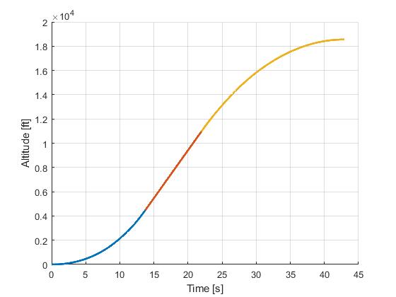
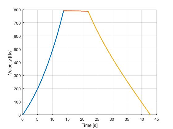
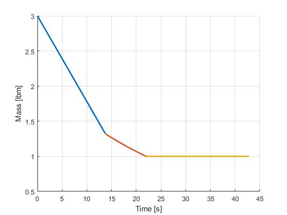
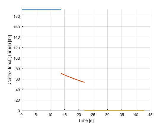
Using the Hermite-Simpson discretization scheme of ICLOCS2, the following state and input trajectories are obtained under a mesh refinement scheme starting with 10 mesh points for each phase. The computation time with IPOPT (NLP convergence tol set to 1e-09) is about 2.5 seconds, using finite difference for derivative calculations on an Intel i7-6700 desktop computer.