Example:
Supersonic Aircraft Minimum Fuel/Time Climb
Difficulty: Intermediate
Aircraft minimum fuel climb problem
The problem was adapted from the supersonic aircraft minimum time-to-climb problem originally presented by [1], formulated by [2] and implemented by [3] in matric units.
Consider following problem aimming at finding a fuel efficient climbing flight path of a supersonic aircraft
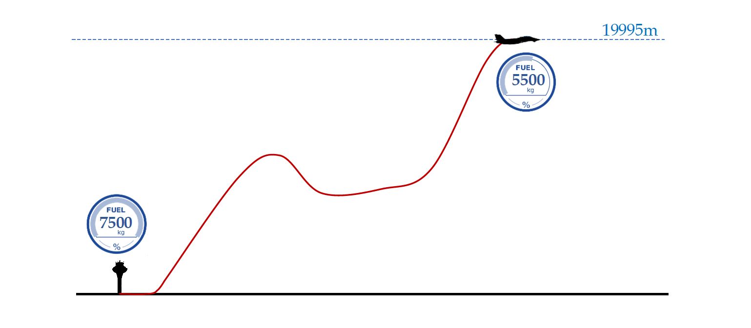
the objective is to maximize the weight of the aircraft at the target altitude

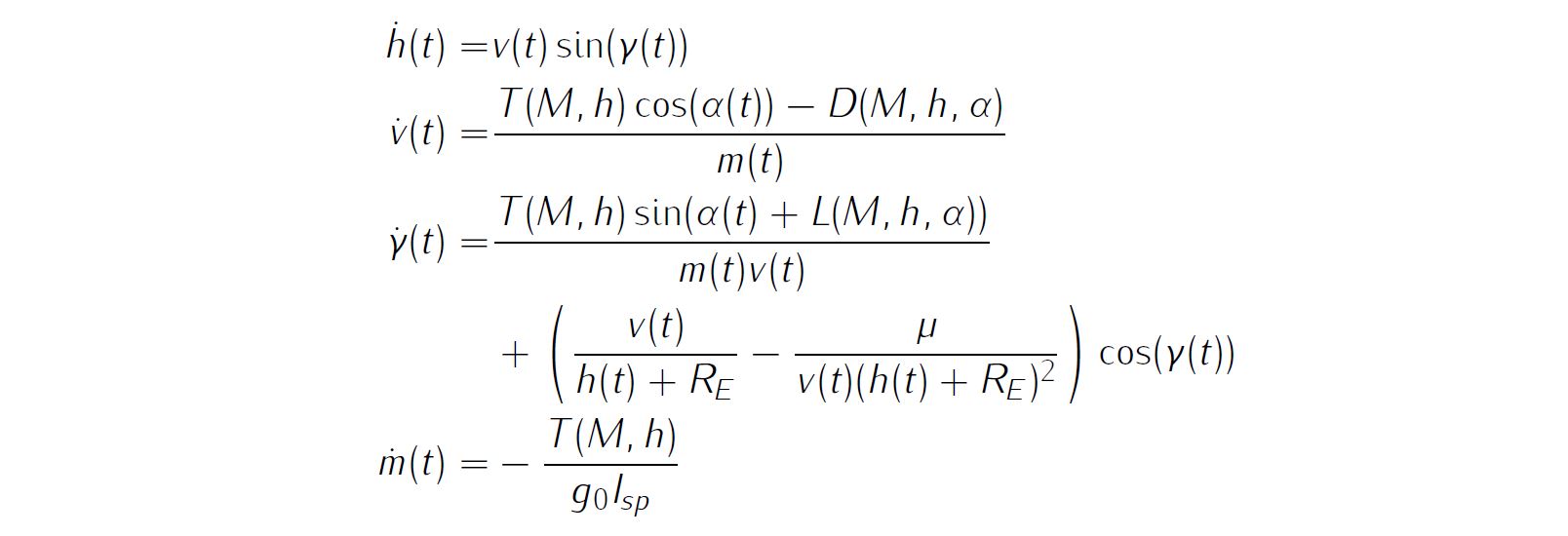
Subject to dynamics constraints
simple bounds on variables

and boundary conditions

Details about the aerodynamic modelling as well as parameter values of all relevant variables are available in various references, thus will not be reproduced here.
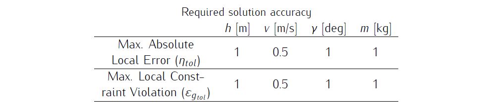
We require the numerical solution to fulfill the following accuracy criteria
Formulate the problem in ICLOCS2
In internal model defination file MinEnergyClimbBryson_Dynamics_Internal.m
We can specify the system dynamics in function MinEnergyClimbBryson_Dynamics_Internal with
Atomsrho = vdat.Atomsrho;
Atomssos = vdat.Atomssos;
TLT = vdat.T;
mu = vdat.mu;
S = vdat.S;
g0 = vdat.g0;
Isp = vdat.Isp;
Re = vdat.Re;

h = x(:,1);
v = x(:,2);
fpa = x(:,3);
mass = x(:,4);
alpha = u(:,1);

r = h+Re;
rho = ppval(Atomsrho,h);
sos = ppval(Atomssos,h);
Mach = v./sos;

CD0 = ppval(vdat.CDdat,Mach);
Clalpha = ppval(vdat.Clalphadat,Mach);
eta = ppval(vdat.etadat,Mach);

Thrust = interp2(vdat.aa,vdat.mm,TLT,h,Mach,'spline');
CD = CD0 + eta.*Clalpha.*alpha.^2;
CL = Clalpha.*alpha;
q = 0.5.*rho.*v.*v;
D = q.*S.*CD;
L = q.*S.*CL;

hdot = v.*sin(fpa);
vdot = (Thrust.*cos(alpha)-D)./mass - mu.*sin(fpa)./r.^2;
fpadot = (Thrust.*sin(alpha)+L)./(mass.*v)+cos(fpa).*(v./r-mu./(v.*r.^2));
mdot = -Thrust./(g0.*Isp);

dx = [hdot, vdot, fpadot, mdot];
For this example problem, we do not have any path constraints, so function MinEnergyClimbBryson_Dynamics_Internal only need to return the value of variable dx .
Similarly, the (optional) simulation dynamics can be specifed in function MinEnergyClimbBryson_Dynamics_Sim.m .
In problem defination file MinEnergyClimbBryson.m
First we need to pre-process the look-up tables of atmosphere data, aerodynamic data and propulsion data for use in ICLOCS2,
% Lookup Table 1: U.S. 1976 Standard Atmosphere (altitude, density and pressure)
AtomsData = [-2000 1.478e+00 3.479e+02
0 1.225e+00 3.403e+02
2000 1.007e+00 3.325e+02
4000 8.193e-01 3.246e+02
6000 6.601e-01 3.165e+02
8000 5.258e-01 3.081e+02
10000 4.135e-01 2.995e+02
12000 3.119e-01 2.951e+02
14000 2.279e-01 2.951e+02
16000 1.665e-01 2.951e+02
18000 1.216e-01 2.951e+02
20000 8.891e-02 2.951e+02
22000 6.451e-02 2.964e+02
24000 4.694e-02 2.977e+02
26000 3.426e-02 2.991e+02
28000 2.508e-02 3.004e+02
30000 1.841e-02 3.017e+02
32000 1.355e-02 3.030e+02
34000 9.887e-03 3.065e+02
36000 7.257e-03 3.101e+02
38000 5.366e-03 3.137e+02
40000 3.995e-03 3.172e+02
42000 2.995e-03 3.207e+02
44000 2.259e-03 3.241e+02
46000 1.714e-03 3.275e+02
48000 1.317e-03 3.298e+02
50000 1.027e-03 3.298e+02
52000 8.055e-04 3.288e+02
54000 6.389e-04 3.254e+02
56000 5.044e-04 3.220e+02
58000 3.962e-04 3.186e+02
60000 3.096e-04 3.151e+02
62000 2.407e-04 3.115e+02
64000 1.860e-04 3.080e+02
66000 1.429e-04 3.044e+02
68000 1.091e-04 3.007e+02
70000 8.281e-05 2.971e+02
72000 6.236e-05 2.934e+02
74000 4.637e-05 2.907e+02
76000 3.430e-05 2.880e+02
78000 2.523e-05 2.853e+02
80000 1.845e-05 2.825e+02
82000 1.341e-05 2.797e+02
84000 9.690e-06 2.769e+02
86000 6.955e-06 2.741e+02];

% Lookup Table 2: Aerodynamic Data
MachLTAero = [0 0.4 0.8 0.9 1.0 1.2 1.4 1.6 1.8];
ClalphaLT = [3.44 3.44 3.44 3.58 4.44 3.44 3.01 2.86 2.44];
CD0LT = [0.013 0.013 0.013 0.014 0.031 0.041 0.039 0.036 0.035];
etaLT = [0.54 0.54 0.54 0.75 0.79 0.78 0.89 0.93 0.93];

% Lookup Table 3: Propulsion Data (Thrust as function of mach number and altitude)
MachLT = [0; 0.2; 0.4; 0.6; 0.8; 1; 1.2; 1.4; 1.6; 1.8];
AltLT = 304.8*[0 5 10 15 20 25 30 40 50 70];
ThrustLT = 4448.2*[24.2 24.0 20.3 17.3 14.5 12.2 10.2 5.7 3.4 0.1;
28.0 24.6 21.1 18.1 15.2 12.8 10.7 6.5 3.9 0.2;
28.3 25.2 21.9 18.7 15.9 13.4 11.2 7.3 4.4 0.4;
30.8 27.2 23.8 20.5 17.3 14.7 12.3 8.1 4.9 0.8;
34.5 30.3 26.6 23.2 19.8 16.8 14.1 9.4 5.6 1.1;
37.9 34.3 30.4 26.8 23.3 19.8 16.8 11.2 6.8 1.4;
36.1 38.0 34.9 31.3 27.3 23.6 20.1 13.4 8.3 1.7;
36.1 36.6 38.5 36.1 31.6 28.1 24.2 16.2 10.0 2.2;
36.1 35.2 42.1 38.7 35.7 32.0 28.1 19.3 11.9 2.9;
36.1 33.8 45.7 41.3 39.8 34.6 31.1 21.7 13.3 3.1];

% Fitting of Aerodynamic data with piecewise splines
Clalphadat = pchip(MachLTAero,ClalphaLT);
CDdat = pchip(MachLTAero,CD0LT);
etadat = pchip(MachLTAero,etaLT);

Atomsrho=pchip(AtomsData(:,1),AtomsData(:,2));
Atomssos=pchip(AtomsData(:,1),AtomsData(:,3));
and declear the variables for later use.
% Boundary Conditions
alt0 = 0;
altf = 19994.88;
speed0 = 129.314;
speedf = 295.092;
fpa0 = 0;
fpaf = 0;
mass0 = 19050.864;

% Simple Bounds
altmin = 0; altmax = 21031.2;
speedmin = 5; speedmax = 1000;
fpamin = -40*pi/180; fpamax = 40*pi/180;
massmin = 22; massmax = 20410;
alphamin = -pi/4; alphamax = pi/4;
Next, we provide the function handles for system dynamics with
InternalDynamics=@MinEnergyClimbBryson_Dynamics_Internal;
SimDynamics=@MinEnergyClimbBryson_Dynamics_Sim;
The optional files providing analytic derivatives can be left empty as we use finite difference this time
problem.analyticDeriv.gradCost=[];
problem.analyticDeriv.hessianLagrangian=[];
problem.analyticDeriv.jacConst=[];
and finally the function handle for the settings file is given as.
problem.settings=@settings_MinEnergyClimbBryson;Next we define the time variables with
problem.time.t0_min=0;
problem.time.t0_max=0;
guess.t0=0;
and
problem.time.tf_min=0;
problem.time.tf_max=400;
guess.tf=324;
For state variables, we need to provide the initial conditions
problem.states.x0=[alt0 speed0 fpa0 mass0];bounds on intial conditions
problem.states.x0l=[alt0 speed0 fpa0 mass0];
problem.states.x0u=[alt0 speed0 fpa0 mass0];
state bounds
problem.states.xl=[altmin speedmin fpamin massmin];
problem.states.xu=[altmax speedmax fpamax massmax];
bounds on the absolute local and global (integrated) discretization error of state variables
problem.states.xErrorTol_local=[0.1 0.1 deg2rad(0.1) 0.1];
problem.states.xErrorTol_integral=[0.1 0.1 deg2rad(0.1) 0.1];
tolerance for state variable box constraint violation
problem.states.xConstraintTol=[0.1 0.1 deg2rad(0.1) 0.1];terminal state bounds
problem.states.xfl=[altf speedf fpaf massmin];
problem.states.xfu=[altf speedf fpaf massmax];
and an initial guess of the state trajectory (optional but recommended)
guess.states(:,1)=[alt0 altf];
guess.states(:,2)=[speed0 speedf];
guess.states(:,3)=[fpa0 fpaf];
guess.states(:,4)=[mass0 mass0];
Lastly for control variables, we need to define simple bounds
problem.inputs.ul=alphamin;
problem.inputs.uu=alphamax;
bounds on the first control action
problem.inputs.u0l=alphamin;
problem.inputs.u0u=alphamax;
tolerance for control variable box constraint violation
problem.inputs.uConstraintTol=deg2rad(0.1); as well as an initial guess of the input trajectory (optional but recommended)
guess.inputs(:,1)=[20 -20]*pi/180;We store the necessary problem parameters used in the functions
problem.data.CDdat = CDdat;
problem.data.Clalphadat = Clalphadat;
problem.data.etadat = etadat;
problem.data.M = MachLT;
problem.data.M2 = MachLTAero;
problem.data.alt = AltLT;
problem.data.T = ThrustLT;
problem.data.Re = 6378145;
problem.data.mu = 3.986e14;
problem.data.S = 49.2386;
problem.data.g0 = 9.80665;
problem.data.Isp = 1600;
problem.data.H = 7254.24;
problem.data.rho0 = 1.225;
problem.data.Atomsrho = Atomsrho;
problem.data.Atomssos = Atomssos;
[aa,mm] = meshgrid(AltLT,MachLT);
problem.data.aa = aa;
problem.data.mm = mm;
Since this problem only has a Mayer (boundary) cost , and no Lagrange (stage) cost ,we simply have
boundaryCost=-xf(4);stageCost = 0*t;for sub-function E_unscaled and L_unscaled respectively.
For this example problem, we do not have additional boundary constraints. Thus we can leave sub-routines b_unscaled as they are.
Main script main_MinEnergyClimbBryson.m
Now we can fetch the problem and options, solve the resultant NLP, and generate some plots for the solution.
[problem,guess]=MinEnergyClimbBryson;          % Fetch the problem definition
% options= problem.settings(10,4);              % for hp method
options= problem.settings(20);                  % for h method
[solution,MRHistory]=solveMyProblem( problem,guess,options);
[ tv, xv, uv ] = simulateSolution( problem, solution, 'ode113', 0.01 );
Note the last line of code will generate an open-loop simulation, applying the obtained input trajectory to the dynamics defined in MinEnergyClimbBryson_Dynamics_Sim.m , using the Matlab builtin ode113 ODE solver with a step size of 0.01.
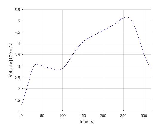
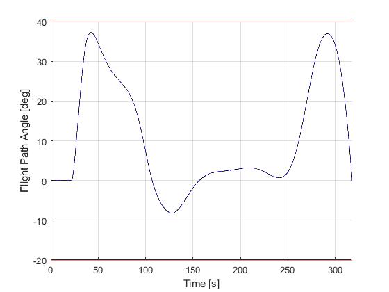
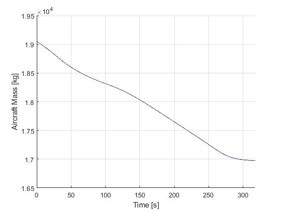
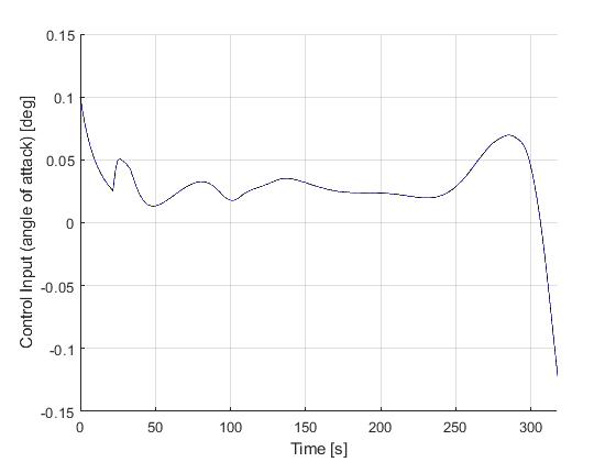
Results from ICLOCS2
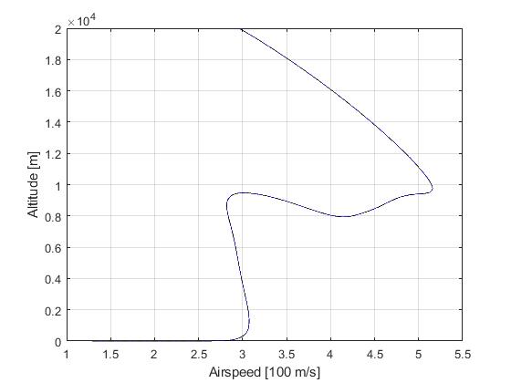
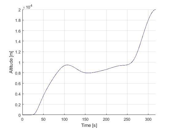
Using the Hermite-Simpson discretization scheme of ICLOCS2, the following state and input trajectories are obtained under a mesh refinement scheme starting with 20 mesh points. The computation time with IPOPT (NLP convergence tol set to 1e-09) is about 9 seconds for 2 mesh refinement iterations together, using finite difference derivative calculations on an Intel i7-6700 desktop computer. Subsequent recomputation using the same mesh and warm starting will take on average 1 seconds and about 10 iterations.
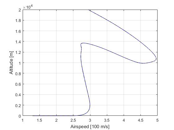
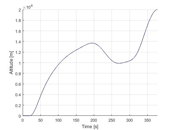
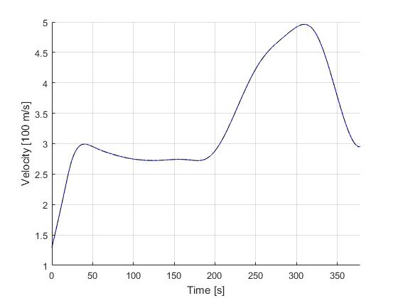
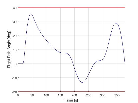
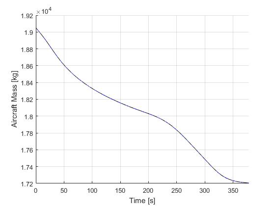
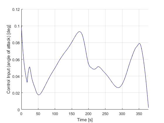
Solution to the minimum time-to-climb problem
The solution to the origial minimum time-to-climb can be obtained by simply changing the objective to

with the obtained solution as follows
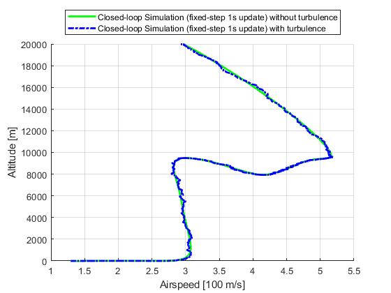
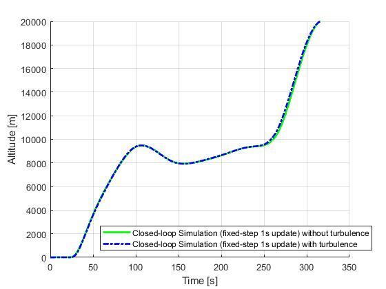
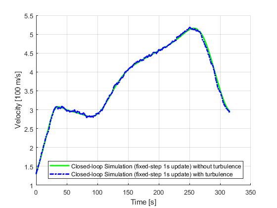
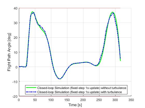
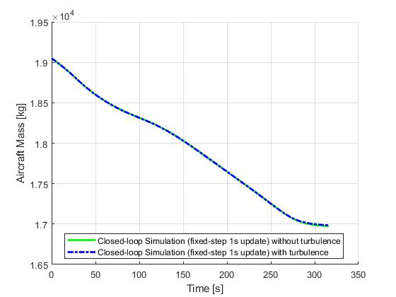
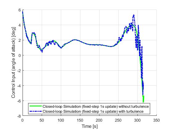
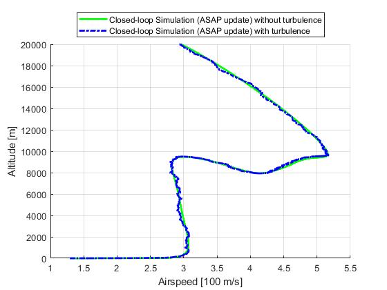
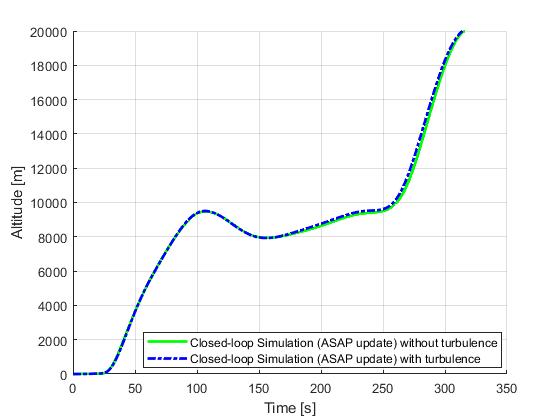
Closed-loop simulation: minimum time-to-climb problem
The followings are the results obtained from various closed-loop simuations of the minimum time-to-climb problem, with and without the perturbations from some atmospheric turbulence. With the shrinking horizon strategy, special attentions was paid to recursive feasiblity of the optimal control problem under uncertainties. For this example, the terminal conditions are implemented as soft constraints, and a lower bound on the terminal time was introduced to avoid numerical issuses with very small time duration (tf-t0 ≈ 0s).
You may use the Link to download the example directly and feel free to use it as a starting point to formulate your own closed-loop simulations.
Fixed-step update
We first demonstrate the results for a fixed-step update strategy. The simulation time step will be 0.1s and the re-optimization time step will be 1s.
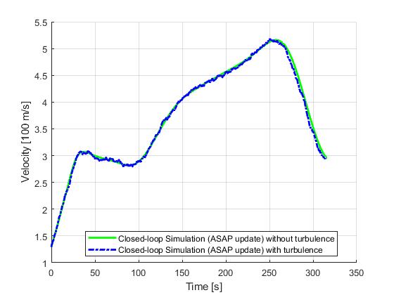
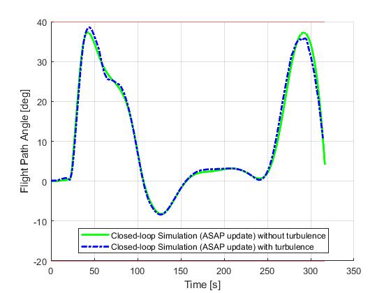
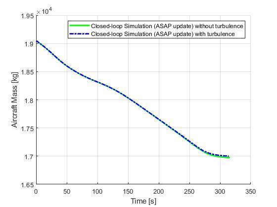
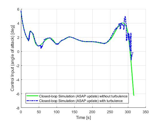
ASAP update
Next, we demonstrate the results for a ASAP update strategy. ASAP stands for 'as soon as possible', meaning each re-optimization solution will become available as soon as the required compuation time has been elapsed.
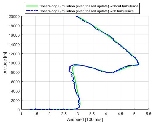
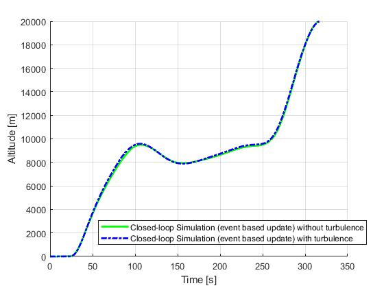
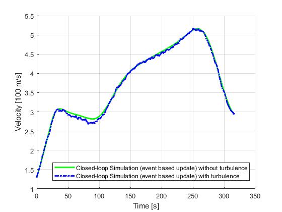
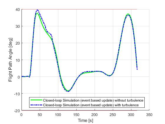
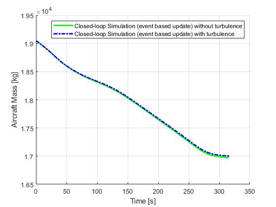
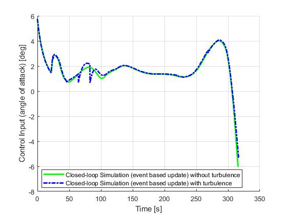
Event based update
Lastly, we present the results for a event-based update strategy. Recomputations will only happy if the previous solution has passed is period of validity (selected to be 20s), or certain variables are close to their upper or lower constraint limits
[1] A. E. Bryson, M. N. Desai, and W. C. Hoffman, Energy-State Approximation in Performance Optimization of Supersonic Aircraft, Journal of Aircraft, Vol. 6, No. 6, November-December, 1969, pp. 481-488.
[2] J. Betts, Practical Methods for Optimal Control and Estimation Using Nonlinear Programming: Second Edition, Advances in Design and Control, Society for Industrial and Applied Mathematics, 2010.
[3] M.A. Patterson and A.V. Rao, GPOPS-II: A General Purpose MATLAB Software for Solving Multiple-Phase Optimal Control Problems, User's Manual, 2.3 edition, 2016.