Example
Double Integrator Tracking of a Sinusoidal Reference Signal
Difficulty: Easy
The problem was adapted from Example 4.11 from [1].
Consider the same system as in Bang-bang control
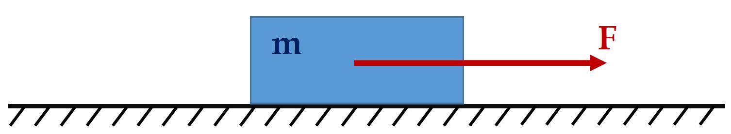
This time, we will formulate an optimal control problem to find the control input trajectory such that the object follows a sine signal for the position, and a cosine signal for the velocity
with Q identify matrix and R=0.0001 for solution uniqueness. The problem need to be solved subject to dynamics constraints

simple bounds on variables
and boundary conditions
We require the numerical solution to fulfill the following accuracy criteria

Formulate the problem in ICLOCS2
In internal model defination file DoubleIntegratorTracking_Dynamics_Internal.m
We can specify the system dynamics in function DoubleIntegratorTracking_Dynamics_Internal with
x2 = x(:,2);
u1 = u(:,1);
dx(:,1) = x2;
dx(:,2) = u1;
For this example problem, we do not have any path constraints, so function DoubleIntegratorTracking_Dynamics_Internal only need to return the value of variable dx .
Similarly, the (optional) simulation dynamics can be specifed in function DoubleIntegratorTracking_Dynamics_Sim.m .
In problem defination file DoubleIntegratorTracking.m
First we provide the function handles for system dynamics with
InternalDynamics=@DoubleIntegratorTracking_Dynamics_Internal;
SimDynamics=@DoubleIntegratorTracking_Dynamics_Sim;
The optional files providing analytic derivatives can be left empty as we demonstrate the use of finite difference this time
problem.analyticDeriv.gradCost=[];
problem.analyticDeriv.hessianLagrangian=[];
problem.analyticDeriv.jacConst=[];
and finally the function handle for the settings file is given as.
problem.settings=@settings_DoubleIntegratorTracking;Next we define the time variables with
problem.time.t0_min=0;
problem.time.t0_max=0;
guess.t0=0;
and
problem.time.tf_min=10;
problem.time.tf_max=10;
guess.tf=10;
For state variables, we need to provide the initial conditions
problem.states.x0=[0 5];bounds on intial conditions
problem.states.x0l=[0 5];
problem.states.x0u=[0 5];
state bounds
problem.states.xl=[-6 -10];
problem.states.xu=[6 10];
bounds on the absolute local and global (integrated) discretization error of state variables
problem.states.xErrorTol_local=[1e-6 1e-6];
problem.states.xErrorTol_integral=[1e-6 1e-6];
tolerance for state variable box constraint violation
problem.states.xConstraintTol=[1e-4 1e-4];terminal state bounds
problem.states.xfl=[-6 -10];
problem.states.xfu=[6 10];
and an initial guess of the state trajectory (optional but recommended)
guess.time=[0 1.5 4.5 8 10];
guess.states(:,1)=[0 5 -5 5 -3];
guess.states(:,2)=[5 0 -1 -1 -5];
Lastly for control variables, we need to define simple bounds
problem.inputs.ul=[-10];
problem.inputs.uu=[10];
bounds on the first control action
problem.inputs.u0l=[-10];
problem.inputs.u0u=[10];
tolerance for control variable box constraint violation
problem.inputs.uConstraintTol=[0.1]; as well as an initial guess of the input trajectory (optional but recommended)
guess.inputs(:,1)=[0 0 0 0 0];Since this problem only has a Lagrange (stage) cost , and no Mayer (boundary) cost ,we simply have
e1=x(:,1)-5.*sin(t);
e2=x(:,2)-5.*cos(t);
u1=u(:,1);
stageCost = e1.*e1+e2.*e2+u1.*u1.*0.0001;boundaryCost=0;for sub-function L_unscaled and E_unscaled respectively.
For this example problem, we do not have additional boundary constraints (in addition to varialbe simple bounds). Thus we can leave routines b_unscaled as it is.
Main script main_DoubleIntegratorTracking.m
Now we can fetch the problem and options, solve the resultant NLP, and generate some plots for the solution.
[problem,guess]=DoubleIntegratorTracking;          % Fetch the problem definition
options= problem.settings(30);                  % Get options and solver settings
[solution,MRHistory]=solveMyProblem( problem,guess,options);
[ tv, xv, uv ] = simulateSolution( problem, solution, 'ode113', 0.01 );
Note the last line of code will generate an open-loop simulation, applying the obtained input trajectory to the dynamics defined in DoubleIntegratorTracking_Dynamics_Sim.m , using the Matlab builtin ode113 ODE solver with a step size of 0.01.
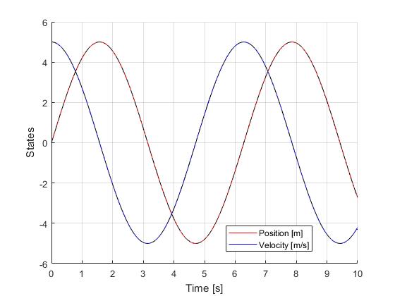
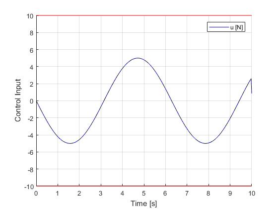
Results from ICLOCS2
Using the Hermite-Simpson discretization scheme of ICLOCS2, the following state and input trajectories are obtained under a mesh refinement scheme starting with 30 mesh points. The computation time with IPOPT (NLP convergence tol set to 1e-09) is about 0.8 seconds with one mesh refinement iteration, using finite difference derivative calculations on an Intel i7-6700 desktop computer. Subsequent recomputation using the same mesh and warm starting will take on average 0.1 seconds and less than 10 iterations.
[1] J. Betts, Practical Methods for Optimal Control and Estimation Using Nonlinear Programming: Second Edition, Advances in Design and Control, Society for Industrial and Applied Mathematics, 2010.