Example: Parallel Parking
Automatic parallel parking in minimum time
Difficulty: Hard
The problem was adapted from [1].
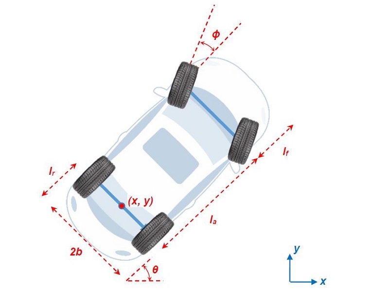
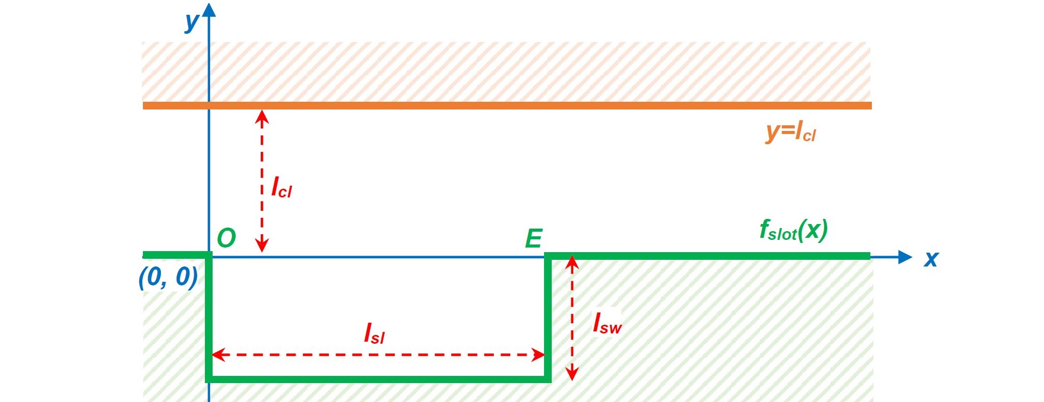
Consider the following geometry of the parking slot
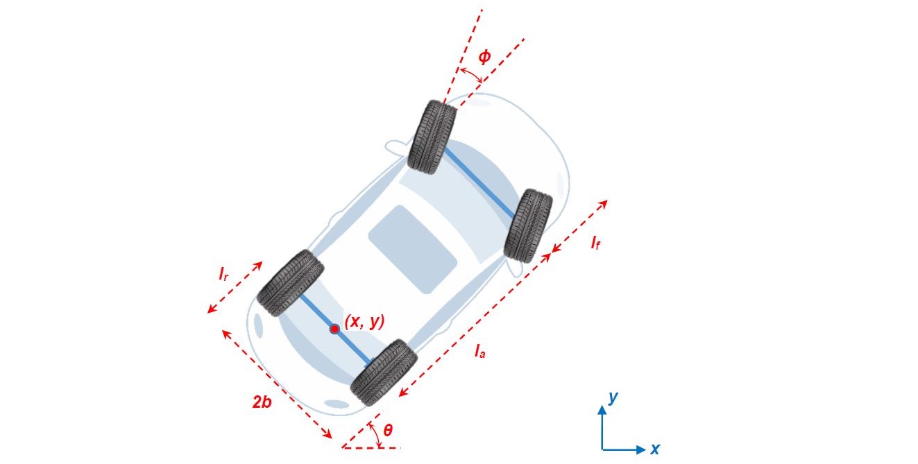
and a generic car model as
the objective is to finish the parallel parking of the car in mimimum time, while requiring the vehicle not to collide with the barriers. Thus we formulate the optimal control problem as

Subject to dynamics constraints

As for path constraints, we first have the ride comfort requirement

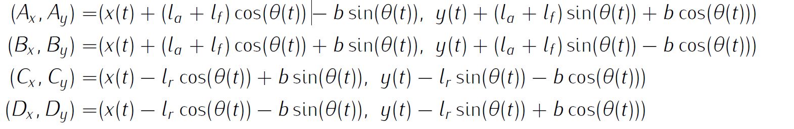
The condition for the vehicle not to collide with the barriers can be approximated by the requirements for the four corners of the car to fulfil the following inequality constraints

with the four corners expressed as
and the lower wall expressed with Heaviside functions as

Nevertheless, there is one exception that the vehicle can still hit the barrier in two corners (point O and E) even when the above conditions are satisfied.
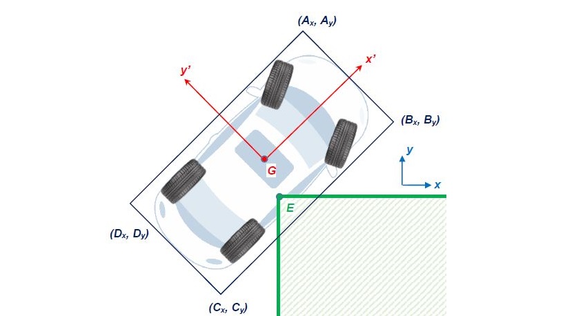
In order to avoid this, the expression of the corner points O and E in vehicle's body frame (x'Gy') are derived.
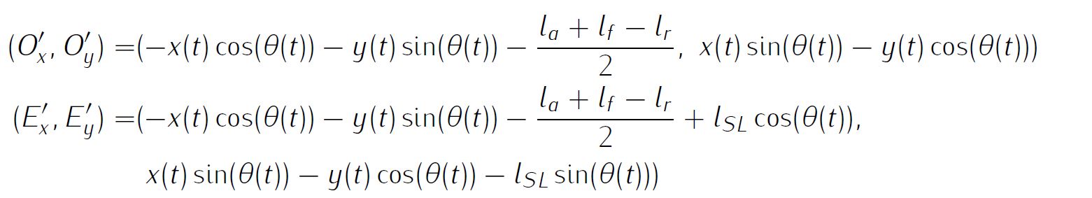
The intuitive implementation of the path constraints for the corners are discontinuous as

which the solver may struggle. Instead, we require equivalently

Additionally we will have simple bounds

and boundary conditions

Details about the parameter values of all relevant variables are available in the reference, thus will not be reproduced here.
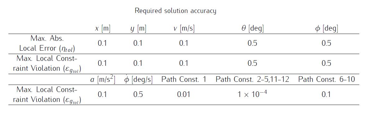
We require the numerical solution to fulfill the following accuracy criteria
Formulate the problem in ICLOCS2
In internal model defination file CarParking_Dynamics_Internal.m
We can specify the system dynamics in function CarParking_Dynamics_Internal with
auxdata = vdat.auxdata;

posx = x(:,1);
posy = x(:,2);
v = x(:,3);
theta = x(:,4);
phi = x(:,5);
a=u(:,1);
u2=u(:,2);

posx_dot=v.*cos(theta);
posy_dot=v.*sin(theta);
v_dot=a;
theta_dot=v.*tan(phi)./auxdata.l_axes;
phi_dot=u2;

pw=vdat.penalty.values(vdat.penalty.i);

curvature_dot=u2./auxdata.l_axes./(cos(phi)).^2;

A_x=posx+(auxdata.l_axes+auxdata.l_front).*cos(theta)-auxdata.b_width.*sin(theta);
B_x=posx+(auxdata.l_axes+auxdata.l_front).*cos(theta)+auxdata.b_width.*sin(theta);
C_x=posx-auxdata.l_rear.*cos(theta)+auxdata.b_width.*sin(theta);
D_x=posx-auxdata.l_rear.*cos(theta)-auxdata.b_width.*sin(theta);

f_p_A_x=(-tanh(pw*(A_x-5/pw))+tanh(pw*(A_x-auxdata.SL+5/pw)))/2.*auxdata.SW;
f_p_B_x=(-tanh(pw*(B_x-0.1))+tanh(pw*(B_x-auxdata.SL+5/pw)))/2.*auxdata.SW;
f_p_C_x=(-tanh(pw*(C_x-0.1))+tanh(pw*(C_x-auxdata.SL+5/pw)))/2.*auxdata.SW;
f_p_D_x=(-tanh(pw*(D_x-0.1))+tanh(pw*(D_x-auxdata.SL+5/pw)))/2.*auxdata.SW;

A_y=posy+(auxdata.l_axes+auxdata.l_front).*sin(theta)+auxdata.b_width.*cos(theta);
B_y=posy+(auxdata.l_axes+auxdata.l_front).*sin(theta)-auxdata.b_width.*cos(theta);
C_y=posy-auxdata.l_rear.*sin(theta)-auxdata.b_width.*cos(theta);
D_y=posy-auxdata.l_rear.*sin(theta)+auxdata.b_width.*cos(theta);

Ox_p=-posx.*cos(theta)-posy.*sin(theta)-(auxdata.l_axes+auxdata.l_front-auxdata.l_rear)/2;
Oy_p=posx.*sin(theta)-posy.*cos(theta);

Ex_p=-posx.*cos(theta)-posy.*sin(theta)-(auxdata.l_axes+auxdata.l_front-auxdata.l_rear)/2+auxdata.SL*cos(theta);
Ey_p=posx.*sin(theta)-posy.*cos(theta)-auxdata.SL*sin(theta);

Ax_p=(auxdata.l_axes+auxdata.l_front+auxdata.l_rear)/2*ones(size(Ox_p));
Ay_p=auxdata.b_width*ones(size(Oy_p));
Bx_p=(auxdata.l_axes+auxdata.l_front+auxdata.l_rear)/2*ones(size(Ox_p));
By_p=-auxdata.b_width*ones(size(Oy_p));
Cx_p=-(auxdata.l_axes+auxdata.l_front+auxdata.l_rear)/2*ones(size(Ox_p));
Cy_p=-auxdata.b_width*ones(size(Oy_p));
Dx_p=-(auxdata.l_axes+auxdata.l_front+auxdata.l_rear)/2*ones(size(Ox_p));
Dy_p=auxdata.b_width*ones(size(Oy_p));

AreaO1=polyarea([Ox_p,Ax_p,Bx_p],[Oy_p,Ay_p,By_p],2);
AreaO2=polyarea([Ox_p,Cx_p,Bx_p],[Oy_p,Cy_p,By_p],2);
AreaO3=polyarea([Ox_p,Ax_p,Dx_p],[Oy_p,Ay_p,Dy_p],2);
AreaO4=polyarea([Ox_p,Dx_p,Cx_p],[Oy_p,Dy_p,Cy_p],2);
AreaO=AreaO1+AreaO2+AreaO3+AreaO4;

AreaE1=polyarea([Ex_p,Ax_p,Bx_p],[Ey_p,Ay_p,By_p],2);
AreaE2=polyarea([Ex_p,Cx_p,Bx_p],[Ey_p,Cy_p,By_p],2);
AreaE3=polyarea([Ex_p,Ax_p,Dx_p],[Ey_p,Ay_p,Dy_p],2);
AreaE4=polyarea([Ex_p,Dx_p,Cx_p],[Ey_p,Dy_p,Cy_p],2);
AreaE=AreaE1+AreaE2+AreaE3+AreaE4;

AreaRef=(auxdata.l_axes+auxdata.l_front+auxdata.l_rear)*2*auxdata.b_width;

%% return dynamics and inequality constraints
dx = [posx_dot, posy_dot, v_dot, theta_dot, phi_dot];
g_neq=[curvature_dot, auxdata.CL-A_y, auxdata.CL-B_y, auxdata.CL-C_y, auxdata.CL-D_y, A_y-f_p_A_x, B_y-f_p_B_x, C_y-f_p_C_x, D_y-f_p_D_x, AreaO-AreaRef, AreaE-AreaRef ];
For this example problem, we have several inequality path constraints, so function CarParking_Dynamics_Internal need to return the value of variable dx and g_neq . Also note that the Heaviside functions are approximated with tanh functions for differentiability.
Similarly, the (optional) simulation dynamics can be specifed in function CarParking_Dynamics_Sim.m . However, for this example problem, the input for directional control of the actual vehicle will be the steering angle instead of the steering rate (in CarParking_Dynamics_Internal ). Therefore, this difference may be reflected in the simulation dynamics and can be easily taken cared of by ICLOCS2.5. We will address this change when calling the simulation function in the main file.
auxdata = data.auxdata;

v = x(:,3);
theta = x(:,4);
phi = u(:,2);
a=u(:,1);

posx_dot=v.*cos(theta);
posy_dot=v.*sin(theta);
v_dot=a;
theta_dot=v.*tan(phi)./auxdata.l_axes;

dx = [posx_dot, posy_dot, v_dot, theta_dot];
In problem defination file CarParking.m
First we provide the function handles for system dynamics with
InternalDynamics=@CarParking_Dynamics_Internal;
SimDynamics=@CarParking_Dynamics_Sim;
The optional files providing analytic derivatives can be left empty as we demonstrate the use of finite difference this time
problem.analyticDeriv.gradCost=[];
problem.analyticDeriv.hessianLagrangian=[];
problem.analyticDeriv.jacConst=[];
and finally the function handle for the settings file is given as.
problem.settings=@settings_CarParking;Next we define the parameters for the scenario,
% Scenario Parameters
SL=5;
SW=2;
CL=3.5;
l_front=0.839;
l_axes=2.588;
l_rear=0.657;
b_width=1.771/2;
phi_max=deg2rad(33);
a_max=0.75;
v_max=2;
u1_max=0.5;
curvature_dot_max=0.6;

% Store data
auxdata.SL=SL;
auxdata.SW=SW;
auxdata.CL=CL;
auxdata.l_front=l_front;
auxdata.l_axes=l_axes;
auxdata.l_rear=l_rear;
auxdata.b_width=b_width;
and declear the variables for later use.
% Boundary Conditions
posx0 = -5.14;
posy0 = 1.41;
theta0=deg2rad(6);
v0=0; % Initial velocity (m/s)
a0=0; % Initial accelration (m/s^2)
phi0 = deg2rad(0); % Initial steering angle (rad)

% Limits on Variables
xmin = -10; xmax = 5;
ymin = -SW; ymax = CL;
vmin = -v_max; vmax = v_max;
amin = -a_max; amax = a_max;
thetamin = -inf; thetamax = inf;
phimin = -phi_max; phimax = phi_max;
Now we may define the time variables with
problem.time.t0_min=0;
problem.time.t0_max=0;
guess.t0=0;
and
problem.time.tf_min=10;
problem.time.tf_max=70;
guess.tf=20;
For state variables, we need to provide the initial conditions
problem.states.x0=[posx0 posy0 v0 theta0 phi0];bounds on intial conditions
problem.states.x0l=[posx0 posy0 v0 theta0 phi0];
problem.states.x0u=[posx0 posy0 v0 theta0 phi0];
state bounds
problem.states.xl=[xmin ymin vmin thetamin phimin];
problem.states.xu=[xmax ymax vmax thetamax phimax];
state rate bounds
problem.states.xrl=[-inf -inf -inf -inf -inf];
problem.states.xru=[inf inf inf inf inf];
bounds on the absolute local and global (integrated) discretization error of state variables
problem.states.xErrorTol_local=[0.1 0.1 0.1 deg2rad(0.5) deg2rad(0.5)];
problem.states.xErrorTol_integral=[0.1 0.1 0.1 deg2rad(0.5) deg2rad(0.5)];
tolerance for state variable box constraint violation
problem.states.xConstraintTol=[0.1 0.1 0.1 deg2rad(0.5) deg2rad(0.5)];
problem.states.xrConstraintTol=[0.1 0.1 0.1 deg2rad(0.5) deg2rad(0.5)];
terminal state bounds
problem.states.xfl=[l_rear ymin 0 theta0-deg2rad(5) -deg2rad(1)];
problem.states.xfu=[SL ymax 0 theta0+deg2rad(5) deg2rad(1)];
and an initial guess of the state trajectory (optional but recommended)
guess.time=[0 guess.tf/3 guess.tf*2/3 guess.tf];
guess.states(:,1)=[posx0 SL+l_rear l_rear SL-l_axes-l_front];
guess.states(:,2)=[posy0 posy0 -SW/2 -SW/2];
guess.states(:,3)=[v0 0 0 0];
guess.states(:,4)=[theta0 theta0 theta0 0];
guess.states(:,5)=[phi0 0 0 0];
Lastly for control variables, we need to define simple bounds
problem.inputs.ul=[amin -curvature_dot_max*l_axes*cos(phimax)^2];
problem.inputs.uu=[amax curvature_dot_max*l_axes*cos(phimax)^2];
bounds on the first control action
problem.inputs.u0l=[amin -curvature_dot_max*l_axes*cos(phimax)^2];
problem.inputs.u0u=[amax curvature_dot_max*l_axes*cos(phimax)^2];
control input rate constraint
problem.inputs.url=[-u1_max -inf];
problem.inputs.uru=[u1_max inf];
tolerance for control variable box constraint and rate constraint violations
problem.inputs.uConstraintTol=[0.1 deg2rad(0.5)];
problem.inputs.urConstraintTol=[0.1 deg2rad(0.5)];
as well as initial guess of the input trajectory (optional but recommended)
guess.inputs(:,1)=[amax amin amax 0];
guess.inputs(:,2)=[0 0 0 0];
Additionally, we need to specify the bounds for the constraint functions . We have no equality path constraint
problem.constraints.ng_eq=0;
problem.constraints.gTol_eq=[];
but do have a number of inequality path constraint
problem.constraints.gl=[-curvature_dot_max 0 0 0 0 0 0 0 0 0 0];
problem.constraints.gu=[curvature_dot_max inf inf inf inf inf inf inf inf inf inf];
problem.constraints.gTol_neq=[deg2rad(0.01) 1e-03 1e-03 1e-03 1e-03 1e-03 1e-03 1e-03 1e-03 1e-03 1e-03];
and boundary constraint function
problem.constraints.bl=[-inf, -inf, -inf, -inf];
problem.constraints.bu=[0 0 0 0];
problem.constraints.bTol=[1e-03 1e-03 1e-03 1e-03];
Next, we may store the necessary problem parameters used in the functions
problem.data.auxdata=auxdata;In version 2.5, ICLOCS can automatically handle the regularization of a variable. For this problem, we want to use hyperbolic tangent functions to approximate the Heaviside functions in the original equation, and make this approximation better and better after the mesh refinement has been complete (with options.regstrategy set to 'MR_priority' in the settings). Here, a sequence for the values of the regularization term can be specified, with the index of the starting value also specified
problem.data.penalty.values=[50 100 150 200];
problem.data.penalty.i=1;
Since this problem only has a Mayer (boundary) cost , and no Lagrange (stage) cost ,we simply have
boundaryCost=tf;stageCost = 0*t;for sub-function E_unscaled and L_unscaled respectively.
Sub-routine b_unscaled for boundary constraints will need to be defined as
auxdata = vdat.auxdata;

posyf = xf(2);
thetaf = xf(4);

A_y=posyf+(auxdata.l_axes+auxdata.l_front).*sin(thetaf)+auxdata.b_width.*cos(thetaf);
B_y=posyf+(auxdata.l_axes+auxdata.l_front).*sin(thetaf)-auxdata.b_width.*cos(thetaf);
C_y=posyf-auxdata.l_rear.*sin(thetaf)-auxdata.b_width.*cos(thetaf);
D_y=posyf-auxdata.l_rear.*sin(thetaf)+auxdata.b_width.*cos(thetaf);

bc=[A_y; B_y; C_y; D_y];
Main script main_CarParking.m
Now we can fetch the problem and options, solve the resultant NLP, and generate some plots for the solution.
[problem,guess]=CarParking;          % Fetch the problem definition
options= problem.settings(200);                  % Get options and solver settings
[solution,MRHistory]=solveMyProblem( problem,guess,options);
[ tv, xv, uv ] = simulateSolution( problem, solution, 'ode113', 0.01,[5;2]);
Note the last line of code will generate an open-loop simulation, applying the obtained input trajectory to the dynamics defined in CarParking_Dynamics_Sim.m , using the Matlab builtin ode113 ODE solver with a step size of 0.01. The last input variable in the syntex is to indicate that the trajectory of the fifth state variable (steering angle) of the optimal control solution is being considered as the second input variable of the simulation dynamics.
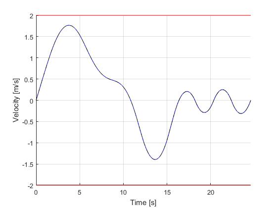
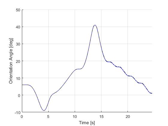
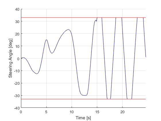
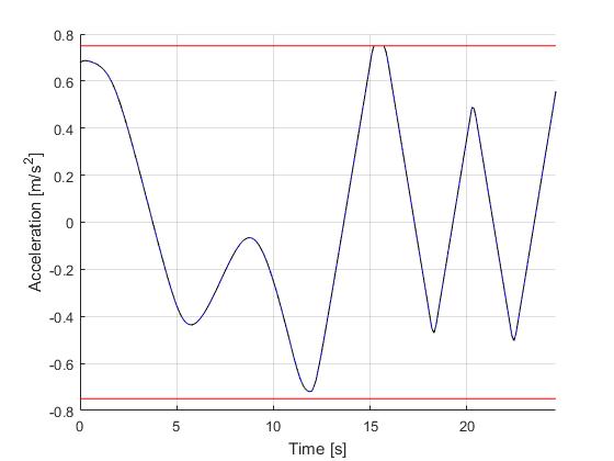
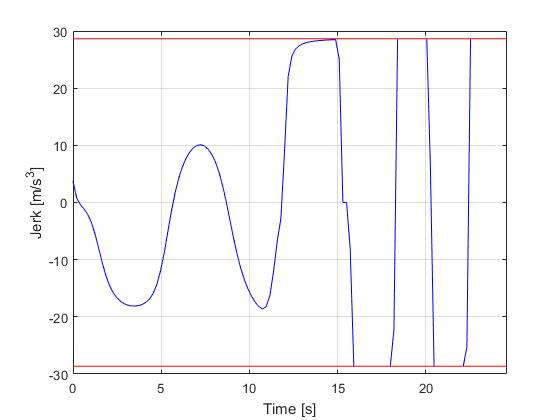
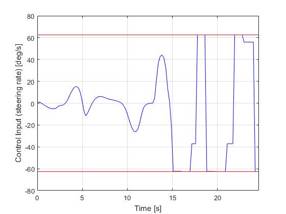
Results from ICLOCS2
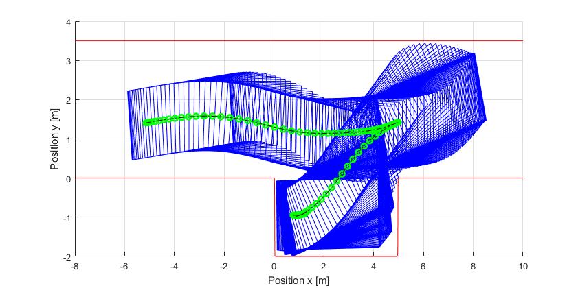
With the existance of singular control in this problem, it is recommended to solve the problem using a realtively dense mesh instead of mesh refinement schemes. This is becasue the fluctuations and ringing phenomena on the singular arc are known to make mesh refinement process diverge. In this case, one often have to make large compromises between solution speed and result accuracy. Here, we focus on the accuracy of the solution.
Using the Hermite-Simpson discretization scheme of ICLOCS2, the following state and input trajectories are obtained using an uniform mesh with 119 intervals. The computation time with IPOPT (NLP convergence tol set to 1e-04) is about 28 seconds , using finite difference derivative calculations on an Intel i7-6700 desktop computer.
[1] B. Li, K. Wang, and Z. Shao, Time-optimal maneuver planning in automatic parallel parking using a simultaneous dynamic optimization approach, IEEE Transactions on Intelligent Transportation Systems, 17(11), pp.3263-3274, 2016.