Example: Low-Thrust Orbit Transfer Problem

Difficulty: Hard

This problem was adapted from Example 6.3 from [1]. This example is available via the link on the right.


The implementation of this examples will not be explained in details due to similarity with other examples. Please refer to an example with similar complexity for implementation instructions, or other examples in the list of examples with Detailed Instructions.

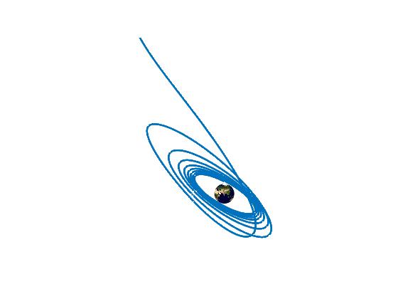
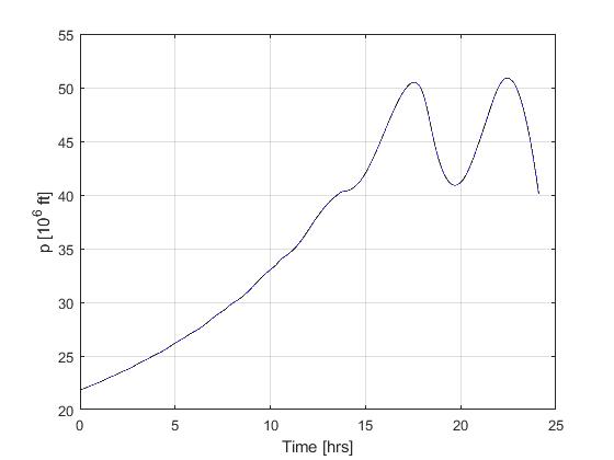
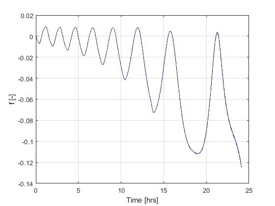
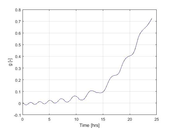
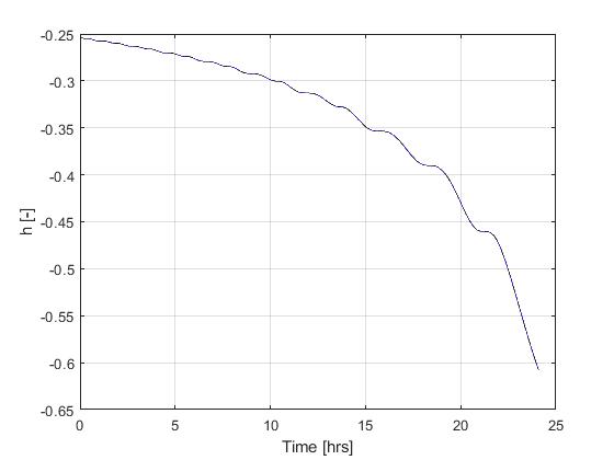
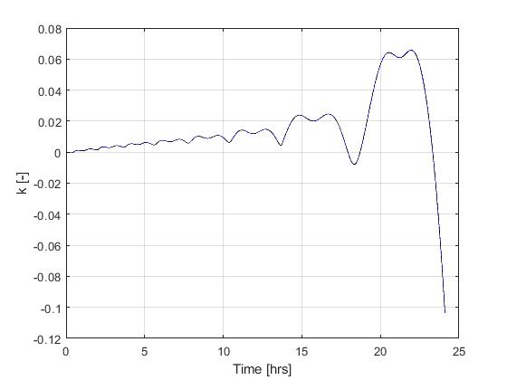
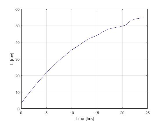
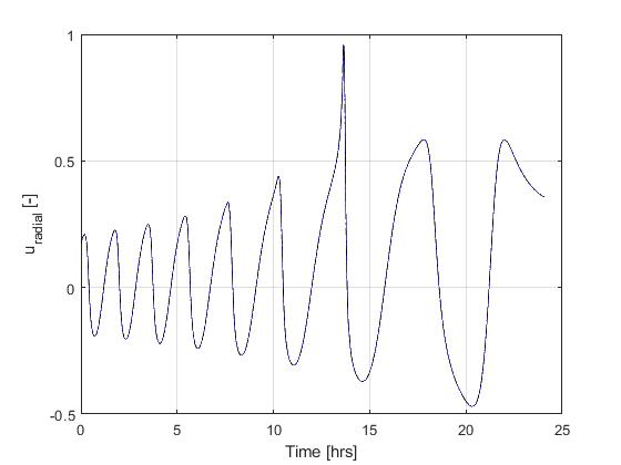
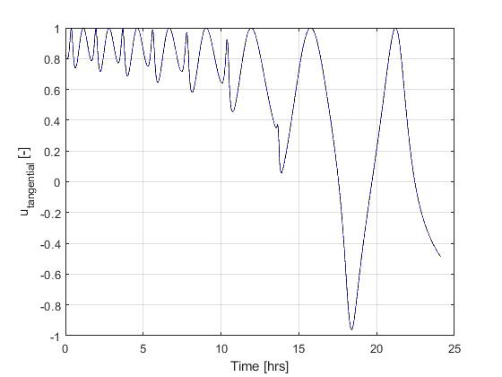
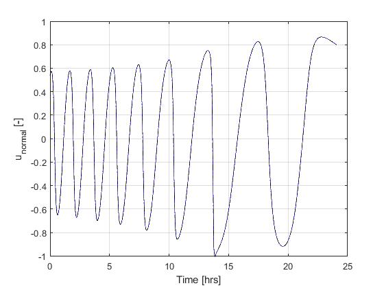
Results from ICLOCS2

Using the Hermite-Simpson discretization scheme of ICLOCS2, the following state and input trajectories are obtained under a mesh refinement scheme starting with 150 mesh points. The relatively large mesh size is due to the large time dimension of the problem (mission duration larger than 24h but dynamics in seconds). The computation time with IPOPT (NLP convergence tol set to 1e-09) is about 373 seconds after 1 mesh refinement iteration, using finite difference derivative calculations on an Intel i7-6700 desktop computer.

Figure 1: Optimal solution for the low-thrust orbit transfer problem
Figure 2: Optimal state (p) trajectory for the low-thrust orbit transfer problem (dash black line indicate the open-loop simulation of the obtained solution)
Figure 3: Optimal state (f) trajectory for the low-thrust orbit transfer problem (dash black line indicate the open-loop simulation of the obtained solution)
Figure 4: Optimal state (g) trajectory for the low-thrust orbit transfer problem (dash black line indicate the open-loop simulation of the obtained solution)
Figure 5: Optimal state (h) trajectory for the low-thrust orbit transfer problem (dash black line indicate the open-loop simulation of the obtained solution)
Figure 6: Optimal state (k) trajectory for the low-thrust orbit transfer problem (dash black line indicate the open-loop simulation of the obtained solution)
Figure 7: Optimal state (L) trajectory for the low-thrust orbit transfer problem (dash black line indicate the open-loop simulation of the obtained solution)
Figure 8: Optimal input (u_r) trajectory for the low-thrust orbit transfer problem (dash black line indicate the open-loop simulation of the obtained solution)
Figure 9: Optimal input (u_t) trajectory for the low-thrust orbit transfer problem (dash black line indicate the open-loop simulation of the obtained solution)
Figure 10: Optimal input (u_n) trajectory for the low-thrust orbit transfer problem (dash black line indicate the open-loop simulation of the obtained solution)

[1] J. Betts, "Practical Methods for Optimal Control and Estimation Using Nonlinear Programming: Second Edition," Advances in Design and Control, Society for Industrial and Applied Mathematics, 2010.