Example: Orbit Raising
Difficulty: Intermediate
The problem was originally presented by [1].
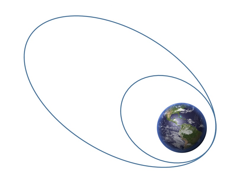
Consider the orbit transfer problem illustrated below
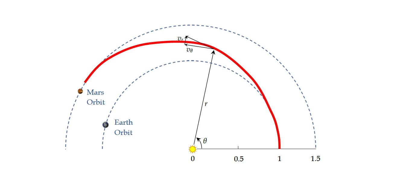
The objective is find the optimal control profile such that radius of the final orbit is maximized:

With scaling and nondimensionalization (e.g. using Astronomical unit), system dynamics can be expressed as

with

Additionally, we have path constraint,

simple bounds on variables,

and boundary conditions

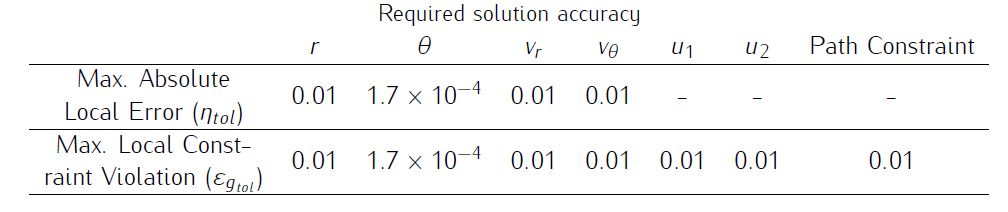
We require the numerical solution to fulfill the following accuracy criteria
Formulate the problem in ICLOCS2
In internal model defination file OrbitRaising_Dynamics_Internal.m
We can specify the system dynamics in function OrbitRaising_Dynamics_Internal with
r=x(:,1);theta=x(:,2);v_r=x(:,3);v_theta=x(:,4);
u_1=u(:,1);u_2=u(:,2);

T1=vdat.T1;
md=vdat.md;
dx=[v_r,v_theta./r,(v_theta.*v_theta)./r-r.^(-2)+(T1./(1-md*t)).*u_1,...
    (-v_r.*v_theta)./r+(T1./(1-md*t)).*u_2];

g_eq=u_1.*u_1+u_2.*u_2-1;
For this example problem, we have one equality path constraints, so function OrbitRaising_Dynamics_Internal need to return the value of variable dx and g_eq .
Similarly, the (optional) simulation dynamics can be specifed in function OrbitRaising_Dynamics_Sim.m .
In problem defination file OrbitRaising.m
First we provide the function handles for system dynamics with
InternalDynamics=@OrbitRaising_Dynamics_Internal;
SimDynamics=@OrbitRaising_Dynamics_Sim;
The optional files providing analytic derivatives can be left empty as we use finite difference this time
problem.analyticDeriv.gradCost=[];
problem.analyticDeriv.hessianLagrangian=[];
problem.analyticDeriv.jacConst=[];
and finally the function handle for the settings file is given as.
problem.settings=@settings_OrbitRaising;Then we may define the time variables with
problem.time.t0_min=0;
problem.time.t0_max=0;
guess.t0=0;
and
problem.time.tf_min=3.32;
problem.time.tf_max=3.32;
guess.tf=3.32;
For state variables, we need to provide the initial conditions
problem.states.x0=[1 0 0 1]; bounds on intial conditions
problem.states.x0l=[1 0 0 1];
problem.states.x0u=[1 0 0 1];
state bounds
problem.states.xl=[0 0 0 0];
problem.states.xu=[2 pi 2 2];
bounds on the absolute local and global (integrated) discretization error of state variables
problem.states.xErrorTol_local=[0.01 deg2rad(0.01) 0.01 0.01];
problem.states.xErrorTol_integral=[0.01 deg2rad(0.01) 0.01 0.01];
tolerance for state variable box constraint violation
problem.states.xConstraintTol=[0.01 deg2rad(0.01) 0.01 0.01]; terminal state bounds
problem.states.xfl=[0 0 0 0];
problem.states.xfu=[2 pi 2 2];
and an initial guess of the state trajectory (optional but recommended)
guess.states(:,1)=[1 1.4];
guess.states(:,2)=[0 2.5];
guess.states(:,3)=[0 0.05];
guess.states(:,4)=[1 0.8];
Lastly for control variables, we need to define simple bounds
problem.inputs.ul=[-1 -1];
problem.inputs.uu=[1 1];
bounds on the first control action
problem.inputs.u0l=[-1 -1];
problem.inputs.u0u=[1 1];
tolerance for control variable box constraint violation
problem.inputs.uConstraintTol=[0.01 0.01]; as well as an initial guess of the input trajectory (optional but recommended)
guess.inputs(:,1)=[0.4 -0.7];
guess.inputs(:,2)=[.9 0.7];
We need to specify the bounds for the constraint functions . We have one equality path constraint
problem.constraints.ng_eq=1;
problem.constraints.gTol_eq=[0.01];
but do not have any inequality path constraint
problem.constraints.gl=[];
problem.constraints.gu=[];
problem.constraints.gTol_neq=[];
Additionally, we have two boundary constraint functions
problem.constraints.bl=[0 0];
problem.constraints.bu=[0 0];
problem.constraints.bTol=[1e-02 1e-02];
We may store the necessary problem parameters used in the functions
problem.data.T1=0.1405;
problem.data.md=0.0749;
Since this problem only has a Mayer (boundary) cost , and no Lagrange (stage) cost ,we simply have
boundaryCost=-xf(1);stageCost = 0*t;for sub-function E_unscaled and L_unscaled respectively.
For this example problem, we do have two boundary constraints (in addition to varialbe simple bounds). Thus we need to specify sub-routines b_unscaled as
bc=[xf(4)-sqrt(1/xf(1));xf(3)];Main script main_OrbitRaising.m
Now we can fetch the problem and options, solve the resultant NLP, and generate some plots for the solution.
[problem,guess]=WindshearGoAround;          % Fetch the problem definition
% options= problem.settings(5,8);                  % for hp method
options= problem.settings(20);                  % for h method
[solution,MRHistory]=solveMyProblem( problem,guess,options);
[ tv, xv, uv ] = simulateSolution( problem, solution, 'ode113', 0.01 );
Note the last line of code will generate an open-loop simulation, applying the obtained input trajectory to the dynamics defined in WindshearGoAround_Dynamics_Sim.m , using the Matlab builtin ode113 ODE solver with a step size of 0.01.
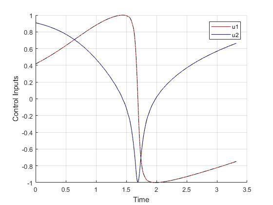
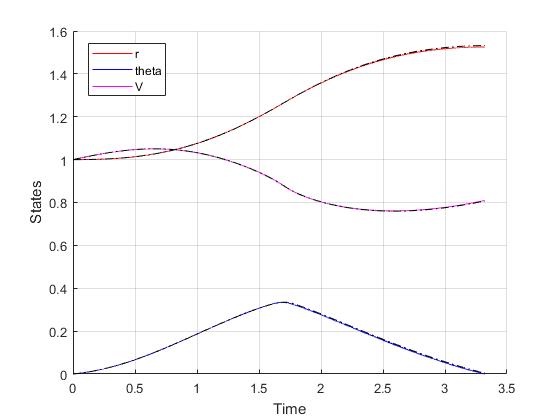
Results from ICLOCS2
Using the Hermite-Simpson discretization scheme of ICLOCS2, the following state and input trajectories are obtained under a mesh refinement scheme starting with 40 mesh points. The computation time with IPOPT (NLP convergence tol set to 1e-09) is about 12 seconds for 2 mesh refinement iterations together, using finite difference derivative calculations on an Intel i7-6700 desktop computer. Subsequent recomputation using the same mesh and warm starting will take on average 0.5 seconds and about 20 iterations.
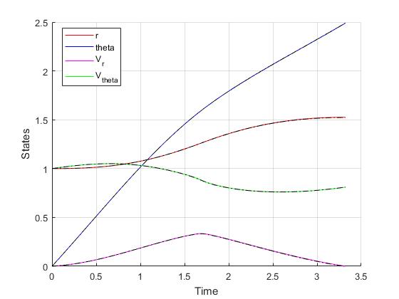
Converting the nondimensionalized time variable back yield

which is equivalent to a journey time of approximately 193 days.
Alternative Formulation
Optimal control problems that are mathematically equivalent may yield different results in compuatational efficiency. Here we demonstrate the benefit of using an alternative formulation of the same orbit raising problem. Instead of using the two elements of the direction vector as control input, we can reformulate the problem that directly uses the directional angle as control inputs. In this way, we can reduce the number of states and inputs by 1 each, and also eliminate the need of one equality path constraint. In addition, faster computations can be obtainable using analytic derivatives infomation rather than finite difference computations.
As the result, using the same Hermite-Simpson discretization with the same 40 mesh points at start, the following state and input trajectories are obtained after refining the mesh 2 time as well. The computation time with IPOPT (NLP convergence tol set to 1e-09) is now reduced to just 1.4 seconds . Subsequent recomputation using the same mesh and warm starting will take on average 0.3 seconds and less than 20 iterations.
[1] A.E. Bryson, and Y.C. Ho, Applied Optimal Control, Hemisphere Publishing, New York, 1975.