ICLOCS2

ICLOCS 2.5 supports closed-loop simulations with a single or multiple MPC controller designs. Each controller should be placed in a separate folder (e.g. MPCController1, MPCController2, etc) and the files in each folder should all have a unique names (e.g. append by 'Phase1', 'Phase2'... for each file). These files are almost identical to the files used in solving a single phase optimal control problem, with the exception that the main file has been replaced by a controller script, ICLOCS_NLPSolver_Phase1.m, for example. In this script, you may pass on the problem definition

[problem,guess]=MyProblem_Phase1;

and configure according to the update strategy. If the optimization resolve is to happen at a fixed interval (defined by opt_step, introduced later), or as soon as the solution is available (by setting opt_step=0), enable the follwing expressions

% Standard Update
if simtime~=0 && simtime>=solution.t_ref+solution.computation_time
    re_opt=1;
end

If a event based strategy would be employed, for example, to resolve the optimization after every 20 seconds, the event triggers can be expressed corrspondingly

% Event Based Update
if simtime>(solution.t_ref+20)
    re_opt=1;
end

another possible trigger could be when certain variables are close to their upper or lower limits

if any(any(x0'>(problem.states.xu-problem.states.xConstraintTol)))
    constVio=x0'-problem.states.xu;
    constVio(constVio<(-problem.states.xConstraintTol))=0;
    if any(constVio)
        re_opt=1;
    end
end
if any(any(x0'<(problem.states.xl+problem.states.xConstraintTol)))
    constVio=problem.states.xl-x0';
    constVio(constVio<(-problem.states.xConstraintTol))=0;
    if any(constVio)
        re_opt=1;
    end
end

Note that the event triggers and standard update can also be employed together.

The plant dynamics can be specified in a sfunction script (e.g. Plant_sfun.m) for simulation with Simulink. First, we need to specify the number of states, inputs and outputs with

sizes.NumContStates  = ...; % Number of states
sizes.NumOutputs     = ...; % Number of outputs
sizes.NumInputs      = ...; % Number of inputs

Then the dynamics equations can be provided in sub-function function [Y,DERX] = Plant_eqn(t,x,u,varargin)

x1 = x(1);
x2 = x(2);
...

u1 = u(1);
...

DERX = [dx1, dx2, ...]; 
Y = [x1, x2, ...]; 

returning two variables: DERX for state derivatives and Y for output variables.

Next, we configure the initialization script (e.g. initSim.m). First, we need to add the MPC controllers to the working path

addpath('MPCController1');
addpath('MPCController2');
...

Then we can configure the time step for simulation, the initial number of mesh points, the function handle for the settings file of the first controller, and fetch the first optimal control problem.

tstep=0.1; % time step of simulation
N_node=20; % initial number of mesh points
settings_func=@settings_MinTimeClimbBryson_Phase1;  % Function handle for the settings file of the first controller
[problem,guess]=MyProblem_Phase1;          % Fetch the problem definition 

Next is to configure the controller function ICLOCS_NLPSolver.m to load different MPC controllers accordingly.

if  ConditionForController2
    opt_step=...; % time interval for re-optimization for controller 2, set to zero for update ASAP
    opt_t_min=0; % stop re-optimizing if solution.tf is smaller than opt_t_min
    [ tfpu ] = ICLOCS_NLPSolver_Phase2(tpx0);
...
else % default controller
    opt_step=0.01; % time interval for re-optimization, set to zero for update ASAP
    opt_t_min=0; % stop re-optimizing if solution.tf is smaller than opt_t_min
    [ tfpu ] = ICLOCS_NLPSolver_Phase1(tpx0);
end

Here, the reoptimization time step opt_step need to be specified for each controller. The value need to be larger than the simulation time step tstep, for a fixed time step re-optimization. Another possibility is to set opt_step=0, using a so called update as soon as possible (ASAP) strategy. In this way, the actual OCP solve time will be recorded and the solution will only become available for update once this time has been elapsed. Another optional setting is opt_t_min, to help alleviate potential issues with very small time duration (tf-t0 ≈ 0s). Once the obtained tf-t0 is smaller than opt_t_min, the optimal control input will be implemented in an open-loop manner without re-optimization.

The last step is to configure the Simulink model Closed_loop_Sim.slx according to the need of different simulations.

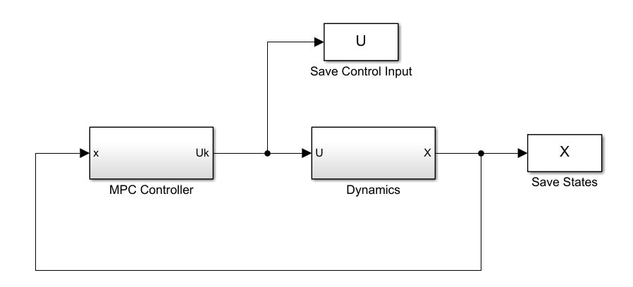
If the simulation plant dynamics sfunction have been given another name, remember to reflect the changes in the Dynamics block. Now make sure the Matlab workspace directory is in the current folder (where you have the initialization script and the Simulink block), and you may run the closed-loop simulation.