Example: Hypersensitive Control
Difficulty: Easy
The problem was originally presented by [1].
Consider the following optimal control problem

subject to dynamics constraint

and boundary conditions

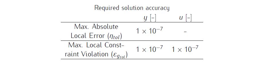
We require the numerical solution to fulfill the following accuracy criteria
Despite the simple formulation, the problem is actually extremely difficult to solve using an indirect method. The state and control near the initial and terminal times experience dramatic changes thus requiring very small stepsizes locally for numerical methods.
Formulate the problem in ICLOCS2
In internal model defination file Hypersensitive_Dynamics_Internal.m
We can specify the system dynamics in function Hypersensitive_Dynamics_Internal with
dx=-x.^3+u;For this example problem, we do not have any path constraints, so function Hypersensitive_Dynamics_Internal only need to return the value of variable dx .
Similarly, the (optional) simulation dynamics can be specifed in function Hypersensitive_Dynamics_Sim.m .
In problem defination file Hypersensitive.m
First we provide the function handles for system dynamics with
InternalDynamics=@Hypersensitive_Dynamics_Internal;
SimDynamics=@Hypersensitive_Dynamics_Sim;
The optional files providing analytic derivatives can be left empty as we demonstrate the use of finite difference this time
problem.analyticDeriv.gradCost=[];
problem.analyticDeriv.hessianLagrangian=[];
problem.analyticDeriv.jacConst=[];
and finally the function handle for the settings file is given as.
problem.settings=@settings_Hypersensitive;Next we define the time variables with
problem.time.t0_min=0;
problem.time.t0_max=0;
guess.t0=0;
and
problem.time.tf_min=10000;
problem.time.tf_max=10000;
guess.tf=10000
For state variables, we need to provide the initial conditions
problem.states.x0=1;bounds on intial conditions
problem.states.x0l=1;
problem.states.x0u=1;
state bounds
problem.states.xl=-inf;
problem.states.xu=inf;
bounds on the absolute local and global (integrated) discretization error of state variables
problem.states.xErrorTol_local=1e-7;
problem.states.xErrorTol_integral=1e-7;
tolerance for state variable box constraint violation
problem.states.xConstraintTol=1e-7;terminal state bounds
problem.states.xfl=1.5;
problem.states.xfu=1.5;
and an initial guess of the state trajectory (optional but recommended)
guess.states(:,1)=[0 0]; Lastly for control variables, we need to define simple bounds
problem.inputs.ul=-inf;
problem.inputs.uu=inf;
bounds on the first control action
problem.inputs.u0l=-inf;
problem.inputs.u0u=inf;
tolerance for control variable box constraint violation
problem.inputs.uConstraintTol=1e-7; as well as an initial guess of the input trajectory (optional but recommended)
guess.inputs(:,1)=[0 0];Since this problem only has a Lagrange (stage) cost , and no Mayer (boundary) cost ,we simply have
stageCost = 0.5*(x.^2+u.^2);boundaryCost=0;for sub-function L_unscaled and E_unscaled respectively.
For this example problem, we do not have additional boundary constraints. Thus we can leave sub-routines b_unscaled as they are.
Main script main_Hypersensitive.m
Now we can fetch the problem and options, solve the resultant NLP, and generate some plots for the solution.
[problem,guess]=Hypersensitive;          % Fetch the problem definition
options= problem.settings(1,8);                  % for hp method
% options= problem.settings(40);                  % for h method
[solution,MRHistory]=solveMyProblem( problem,guess,options);
[ tv, xv, uv ] = simulateSolution( problem, solution, 'ode113', 0.01 );
Note the last line of code will generate an open-loop simulation, applying the obtained input trajectory to the dynamics defined in Hypersensitive_Dynamics_Sim.m , using the Matlab builtin ode113 ODE solver with a step size of 0.01.
Results from ICLOCS2
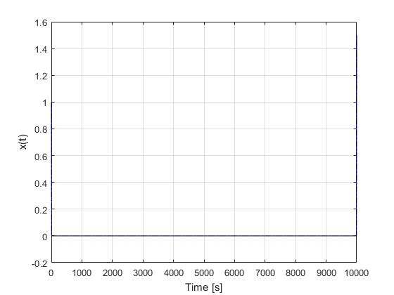
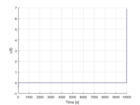
Using the hp-LGR discretization scheme of ICLOCS2, the following state and input trajectories are obtained under a mesh refinement scheme starting with 1 mesh interval with polynomial order of 8. The computation time with IPOPT (NLP convergence tol set to 1e-09) is about 1 seconds for 4 mesh refinement iterations together, using finite difference derivative calculations on an Intel i7-6700 desktop computer. The final mesh have 43 intervals with polynomial orders ranging from 3 to 8. Subsequent recomputation using the same mesh and warm starting will take on average 0.1 seconds and about 3 iterations.
It is interesting to note that if this problem is to be solved without the mesh refinement scheme using equally spaced mesh, even 1000 grid intervals with the same polynomial order can only bring down the maximum absolute local error to 0.6273, far larger than the required 0.0000001. The computation time in this case is about 15 seconds (14900% higher). This clearly demonstrated the benefit and necessity of mesh refinement .
[1] A.V. Rao, and K.D. Mease, Eigenvector approximate dichotomic basis method for solving hyper-sensitive optimal control problems, Optimal Control Applications and Methods, 21(1), pp.1-19, 2000.